2D FDTD wave simulation

Most of phonometry predicts a number: a level, a reverberation time, a transmission loss. The simulation domain computes the wave field itself: fdtd_simulation integrates the linear acoustic equations on a 2D grid with the finite-difference time-domain (FDTD) method, so reflection, diffraction, interference, refraction through inhomogeneous media and modal behaviour all emerge from first principles instead of being modelled term by term. The implementation follows the reference formulation for outdoor sound of Attenborough & Van Renterghem, Predicting Outdoor Sound (2nd ed., CRC Press 2021), chapter 4: the staggered-in-place, staggered-in-time pressure-velocity scheme (Eqs. 4.11-4.12), the Courant stability condition (Eqs. 4.13-4.14), rigid boundaries as zero normal face velocity (Eq. 4.32) and the frequency-independent real-impedance boundary (Eqs. 4.33-4.35).

The solver is deterministic by design: float64 arithmetic, no random numbers and single-threaded numpy stepping, so the same inputs produce bit-identical outputs on the same platform. It is the engine behind the FDTD animations of this documentation, promoted to a public API with sources, pressure probes, rasterised obstacles, per-side boundary conditions and a frozen result object.

Here is one of those animations, and it is a fair advertisement for what the rest of this page builds. Nothing in it is drawn: the colonnade is a boolean obstacle_mask of rasterised circles and the wavefront is a single one-way plane-wave packet with a Gaussian envelope one wavelength wide, launched at $x=0.30$ m into a 4 m × 1 m rigid-walled hall whose two ends absorb through sponges hidden outside the frame. The carrier is 800 Hz, so the wavelength is 42.9 cm and the 10 to 17 cm columns are roughly a quarter to two fifths of it — the regime in which a rigid cylinder both casts a readable shadow and re-radiates strongly, which is why the coda that fills the hall is structured rather than noise. That coda is deterministic multiple scattering: it is what a diffuse field looks like before any statistical assumption is made about it. The mesh is the worked example of the rule section 6 derives: the tightest gap in this layout is 6.6 cm between a column and a wall, so $\Delta x=\min (\text{smallest aperture}/4,\lambda /8)$ allows up to 1.6 cm, and the clip runs at 2.5 mm because a banner needs the definition.

An 800 Hz plane wavefront sweeps a 4 m rigid-walled hall filled with a staggered colonnade of rigid columns 10 to 17 cm across, simulated at 2.5 mm; every column diffracts the front and sheds a scattered wavelet, and the wavelets interfere until the whole hall is filled with structured energy that then drains through the absorbing ends.

Download the animation (WebM)

An 800 Hz plane wavefront sweeps a 4 m rigid-walled hall filled with a staggered colonnade of rigid columns 10 to 17 cm across, simulated at 2.5 mm; every column diffracts the front and sheds a scattered wavelet, and the wavelets interfere until the whole hall is filled with structured energy that then drains through the absorbing ends.

Download the animation (WebM)

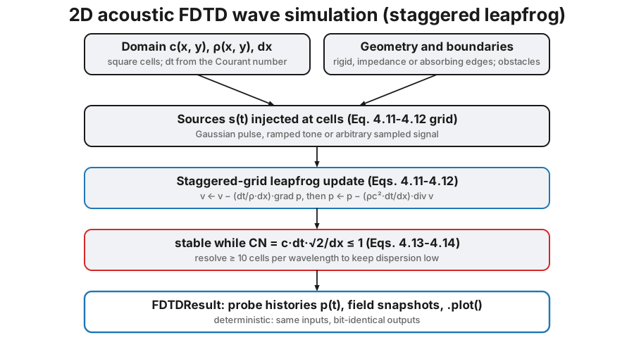
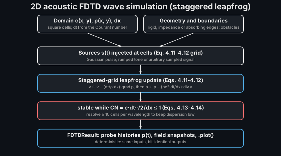
1. The scheme: a wave equation on a grid

In a non-moving medium the linearised equations of fluid dynamics reduce to a first-order system in the acoustic pressure $p$ and particle velocity $\mathbf{v}$ (Attenborough & Van Renterghem Eqs. 4.3-4.4):

$$\frac{\partial p}{\partial t}+\rho c^2\nabla \cdot \mathbf{v}=0,\frac{\partial \mathbf{v}}{\partial t}+\frac{1}{\rho }\nabla p=0.$$

FDTD discretises both on a staggered grid (the acoustic analogue of the Yee cell): pressure lives at cell centres and each velocity component on the cell faces, half a cell away, and the two fields leapfrog in time, half a time step apart (Eqs. 4.11-4.12). Evaluating each spatial gradient exactly where the other field needs it gives a fourfold accuracy gain over a collocated grid (Eq. 4.9 vs 4.10) and allows in-place updates. Because only interior faces are stored, the domain edge is a perfectly rigid wall (zero normal velocity, Eq. 4.32) unless another boundary is requested.

The explicit scheme is stable only while a wavefront crosses at most one cell per time step. With square cells the Courant number (Eq. 4.13) is

$$\mathrm{CN}=c\Delta t\sqrt{\frac{1}{\Delta x^2}+\frac{1}{\Delta y^2}}=\frac{c\Delta t\sqrt{2}}{\Delta x}\le 1,$$

and fdtd_simulation derives the time step from the cfl parameter (this $\mathrm{CN}$, default 0.6) and the largest sound speed in the map. The scheme is only conditionally stable: at $\mathrm{CN}\le 1$ the update neither creates nor destroys energy, and above the bound every mode with a wavelength near the grid scale grows exponentially, so the run reaches inf within a few hundred steps rather than degrading gracefully (Eq. 4.14). fdtd_simulation therefore rejects any cfl outside $(0,1)$ instead of letting the run start. Section 6 also uses a per-axis Courant number $S=c\Delta t/\Delta x=\mathrm{CN}/\sqrt{2}$ in the dispersion relation; the two are not the same number, and the default cfl = 0.6 means $S=0.424$.

from phonometry import simulation

# A 3.0 x 2.0 m air domain: 300 x 200 cells of 1 cm.
res = simulation.fdtd_simulation(
    343.0,             # c: sound speed [m/s], a scalar or a map over the grid
    0.01,              # dx: square cell size [m]
    2.0e-3,            # duration: simulated time [s] (dt is derived, not given)
    shape=(200, 300),  # (ny, nx) cells -> a 2.0 x 3.0 m domain
    sources=[simulation.GaussianPulse(ix=60, iy=100, width=3.0e-4)],
    probes=[(200, 100)],
)
print(res.size)                  # (3.0, 2.0)  metres
print(round(res.dt * 1e6, 2))    # 12.37  microseconds (CN = 0.6)
res.plot()                       # probe pressure histories (figure in section 5)

The time step is not an input. It follows from cfl and the largest sound speed in the map, and res.dt reports the value that was used — which is why the duration is given in seconds of simulated time and never in steps.

The grid is index-based: cell (ix, iy) has its centre at ((ix + 0.5) * dx, (iy + 0.5) * dx) metres, with rows plotted downward (the imshow convention), so a position in metres maps to ix = round(x / dx - 0.5).

2. Sources, probes, obstacles and boundaries

Three source types inject a soft source (an additive pressure contribution that does not scatter passing waves) at a grid cell: GaussianPulse (a broadband pulse of temporal half-width width), CWSource (a sine tone faded in with a raised-cosine ramp so its onset does not splash a broadband transient) and SignalSource (an arbitrary sampled waveform, linearly interpolated onto the simulation time steps). Probes record the pressure at their cell every time step into the result.

Plane waves “from infinity”. Point sources in 2D are really line sources, so a diffuser or a barrier is often better interrogated with a plane wavefront. Two tools cover it, each one-way through its own mechanism:

• sim.add_plane_wave(direction, center=..., width=..., wavelength=...) superimposes a Gaussian packet (optionally carrying a sine) as an initial condition travelling toward "down", "up", "left" or "right"; the leapfrog-consistent velocity written half a step back is what makes it one-way, and behind the front the residual energy is at numerical noise level. This is what the QRD diffusion animation uses.
• PlaneWaveSource(direction, waveform, offset=...) registered through add_source() injects a sustained plane wave on a line of cells: the incident pressure and the adjacent face velocity are driven together, so the launched field is transversely plane to machine precision and anything scattered back crosses the line untouched; with a sponge configured behind the line it is then absorbed.

from phonometry.simulation import FDTD2D, CWSource, PlaneWaveSource

sim = FDTD2D(343.0, 0.01, shape=(160, 80), sponge_width=20,
             sponge_sides=("top", "bottom"))
tone = CWSource(0, 0, frequency=1000.0)          # reused as a waveform
sim.add_source(PlaneWaveSource("down", tone.value, offset=22))
# or, for a single packet: sim.add_plane_wave("down", center=0.4,
#                                             width=0.08, wavelength=0.34)

Both quantitative claims in that bullet are measurable, and the figure below measures them on exactly this scene. “Transversely plane to machine precision” is literal: after the fill transient every column of the settled field carries the same float64 value, so the largest difference across a row is 0.0 and not merely small. “One-way” is not: the injection line leaks a little backwards, and what is left behind it is only small because the sponge is there to eat it — 1.4 × 10⁻⁴ of the field energy, that is −38.4 dB, sits in the 20 sponge rows behind the line, but immediately behind the line itself the pressure is only about 26 dB down on the forward wave. Move the line away from its sponge, or forget the sponge, and that 26 dB is what comes back at you.

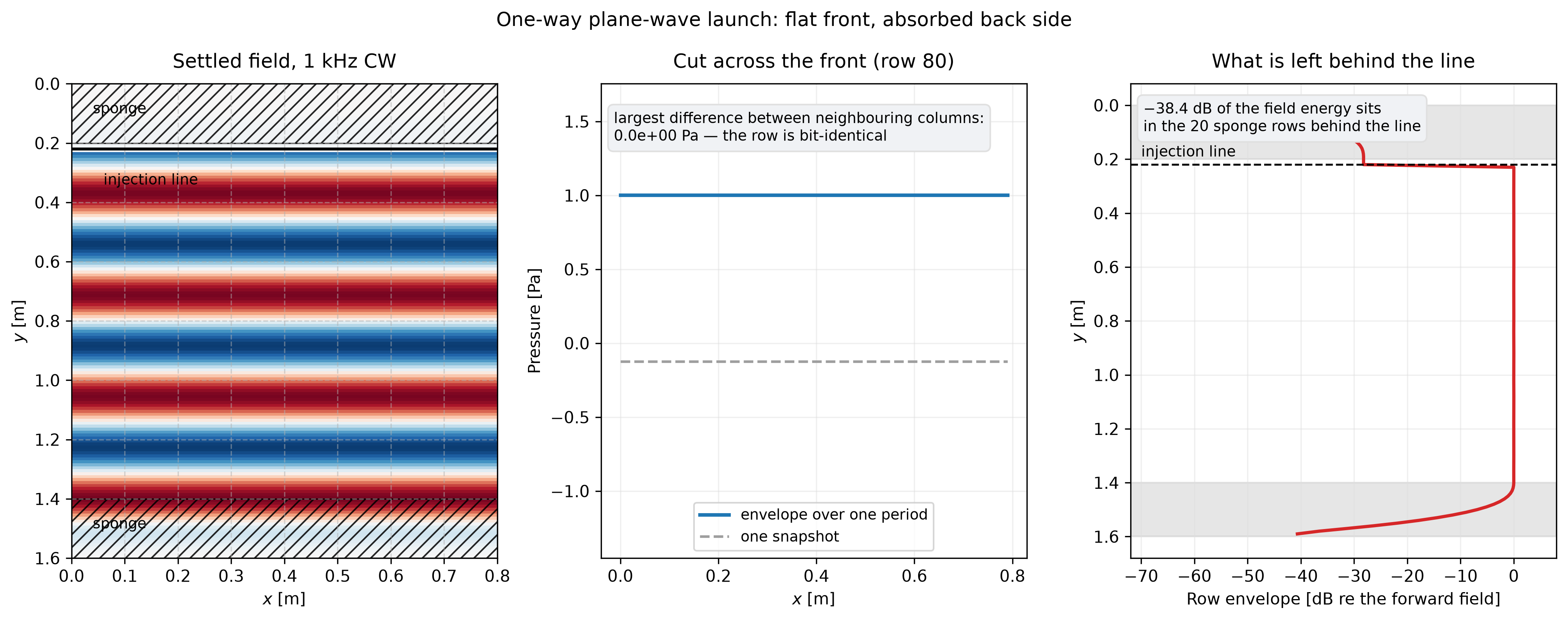
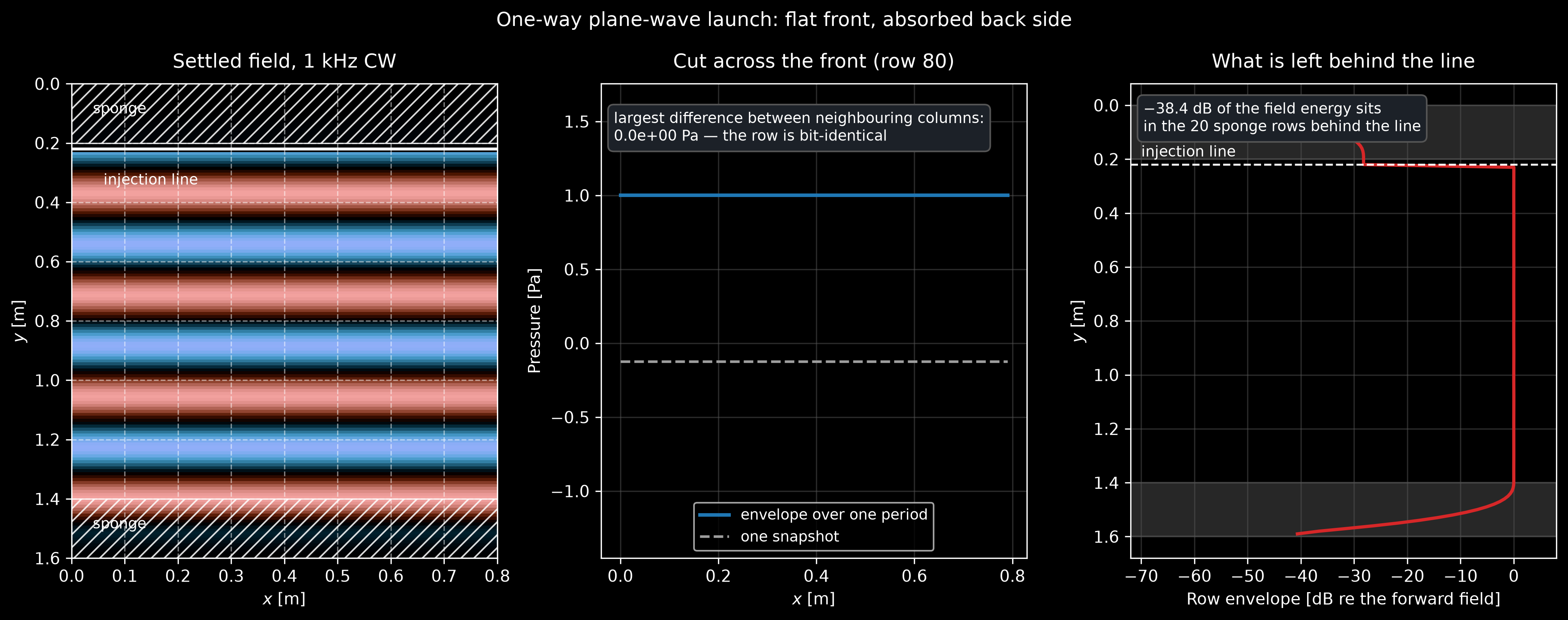
What a correctly configured one-way launcher looks like: the front is flat to the last bit of a float64 (centre), the forward field holds unit amplitude, and the residual behind the injection line starts 26 dB down and is buried by the sponge that side is carrying (right). The sponge is not an optional tidy-up — without it the back-side residual reflects off the top edge and comes back through the measurement.

Show the code for this figure

import numpy as np
import matplotlib.pyplot as plt

# `FDTD2D`, `CWSource` and `PlaneWaveSource` are the names imported above.
sim = FDTD2D(343.0, 0.01, shape=(160, 80), sponge_width=20,
             sponge_sides=("top", "bottom"))
sim.add_source(PlaneWaveSource(
    "down", CWSource(0, 0, frequency=1000.0).value, offset=22))
sim.run(700)                                   # ramp + fill + a few periods

body = sim.p[60:140, :]
print(float(np.abs(np.diff(body, axis=1)).max()))     # 0.0  exactly plane
back = float((sim.p[:20, :] ** 2).sum()) / float((sim.p ** 2).sum())
print(round(10 * np.log10(back), 1))                  # -38.4  dB of energy

rms = np.sqrt((sim.p ** 2).mean(axis=1))
fig, (ax_f, ax_t, ax_l) = plt.subplots(1, 3, figsize=(13.5, 5.0))
ax_f.imshow(sim.p, cmap="RdBu_r", vmin=-1.05, vmax=1.05)
ax_t.plot(sim.p[80, :])                               # transverse cut
ax_l.plot(20 * np.log10(rms / rms[60:140].mean()), np.arange(160))
plt.show()

Geometry is rasterised: obstacle_mask marks rigid cells, and every face touching a masked cell is closed (Eq. 4.32 again), so walls, barriers and scatterers of any shape are just boolean arrays. A face is either open or closed, with nothing in between, so a surface that runs along a grid axis is represented exactly and every other surface becomes a staircase whose steps are one cell tall. Those steps scatter energy the real surface does not, they displace the effective surface by up to half a cell, and — because the error is a fixed fraction of a cell rather than of a wavelength — it does not shrink as the wave gets longer. It is worst at grazing incidence and at the top of the resolved band. The working rule is that a tilted or curved reflector needs a finer grid than the ten-cell dispersion rule alone would ask for, with the same diagnostic as for dispersion: halve $\Delta x$ and confirm that the scattered field converges rather than merely changing. That is why the meshed panel of section 4 runs at half a millimetre, far finer than its 17 cm wavelength requires — there the geometry, not the wavelength, sets the resolution.

Each domain side can carry its own boundary condition:

• "rigid" (default): a perfect reflector, $R=+1$.
• "absorbing": a sponge layer of absorbing_layer_cells cells whose absorption rate ramps quadratically, emulating an open boundary (the simple precursor of the perfectly matched layers of Attenborough & Van Renterghem section 4.2.3).
• a real specific impedance $Z$ in Pa·s/m (a scalar or one value per edge cell): the locally reacting boundary of Eqs. 4.33-4.35, updated implicitly, with the normal-incidence reflection coefficient $R=(Z-\rho c)/(Z+\rho c)$; $Z=\rho c$ is anechoic.

The two facilities are not interchangeable, and only one of them is soft. The four domain sides can be rigid, sponge or a locally reacting real impedance; anything drawn in obstacle_mask is perfectly rigid by construction. A room modelled as interior walls inside a larger domain therefore has hard walls whatever the edges do, and there is no way to hand an interior surface an absorption coefficient. Two routes soften a surface: put it on a domain edge and give that edge an impedance, or back it with a lossy region through the damping map below. When an edge will do, the conversion from a target normal-incidence absorption coefficient is two steps — the reflection magnitude is $|R|=\sqrt{1-\alpha }$, and for a real impedance $Z=\rho c(1+R)/(1-R)$, so $\alpha =0.5$ needs $Z\approx 5.83\rho c$ and $\alpha =0.9$ about $1.92\rho c$. The caveat comes with it: $R$ is exact only at normal incidence, so a locally reacting edge absorbs less as the incidence gets more oblique and a room bounded by such edges decays more slowly than its nominal $\alpha$ suggests.

Volumetric loss: the damping map. damping is a per-cell amplitude decay rate $\sigma$ in s⁻¹, applied to the pressure and to both velocity components at once. Because both fields decay together, a plane wave inside a uniform lossy region follows $k=(\omega -j\sigma )/c$: the amplitude falls exponentially in space at $\sigma /c$ nepers per metre while the characteristic impedance stays real at $\rho c$. That is an equivalent fluid — same sound speed, same density, frequency-independent loss — and it is the only volumetric loss the solver has, hence also the only way to make an interior surface absorb. Two routes to a value. As a stand-in for room absorption, $\sigma =6.91/T_{60}$ produces a $T_{60}$-second reverberant decay, so a 0.5 s decay is $\sigma =13.8$ s⁻¹. As a sample, the loss per metre is $\sigma /c$ nepers ($8.69\sigma /c$ dB/m), and the value is tuned until the modelled sample reproduces a measured absorption. The two limits are worth stating plainly: because the loss is frequency-independent and the impedance stays real, this is not a Delany-Bazley or Johnson-Champoux-Allard model and will not reproduce a real absorber’s frequency dependence; and FDTD2D accepts a scalar or an (ny, nx) map, while the convenience fdtd_simulation takes a scalar only, so a region-by-region absorber has to be built on the engine.

import numpy as np

# A three-row lossy duct: the decay per metre is the whole of the model.
# (`simulation` is the name section 1 imported.)
sigma = 200.0                                     # amplitude decay rate [1/s]
lossy = simulation.FDTD2D(343.0, 0.01, shape=(3, 900), damping=sigma)
x = (np.arange(900) + 0.5) * 0.01
lossy.p[:] = np.exp(-(((x - 1.0) / 0.15) ** 2))[None, :]
peaks = []
for _ in range(round(0.020 / lossy.dt)):
    lossy.step()
    peaks.append((lossy.p[1, 200], lossy.p[1, 500]))
peaks = np.abs(np.asarray(peaks))
print(round(float(peaks[:, 1].max() / peaks[:, 0].max()), 3))  # 0.173
print(round(float(np.exp(-sigma * 3.0 / 343.0)), 3))           # 0.174 exact
print(round(8.686 * sigma / 343.0, 2))         # 5.06 dB per metre
print(round(6.91 / 13.82, 2))                  # 0.5 s of T60 at sigma = 13.82

The calibrated route is at the end of this section: the impedance-tube guide drives this same solver with a damping map and puts the result through the ISO 10534-2 reduction, so the modelled sample’s absorption comes back out of a virtual measurement rather than out of the value that went in.

The stepping engine FDTD2D is public too: it exposes step(), run(), the field arrays and the energy, for callers that need frame-by-frame access (the documentation animations use it directly). A plane pulse launched down a duct against an impedance edge reproduces the textbook reflection coefficient:

import numpy as np
from phonometry import simulation

rho, c, dx = 1.2, 343.0, 0.01
sim = simulation.FDTD2D(c, dx, rho=rho, shape=(3, 1200),
                        edge_impedance={"right": 3.0 * rho * c})
x = (np.arange(1200) + 0.5) * dx
sim.p[:] = np.exp(-(((x - 6.0) / 0.15) ** 2))[None, :]   # plane pulse

trace = []
for _ in range(int(round(0.032 / sim.dt))):
    sim.step()
    trace.append(sim.p[1, 900])
trace = np.asarray(trace)
t = (np.arange(trace.size) + 1) * sim.dt
t_return = 6.0 / c + 3.0 / c                  # via the wall, back to x = 9 m
incident = trace[t < t_return - 0.001].max()
echo = trace[t > t_return]
print(round(float(echo[np.abs(echo).argmax()] / incident), 2))  # 0.5
# (Z - rho c)/(Z + rho c) = (3 - 1)/(3 + 1) = +0.5

Before spending a single time step, sim.plot_geometry() draws the configured domain: edges, sponges, obstacles, sources and the probes you intend to record. Catching a sponge on the wrong side or a probe in the wrong place costs seconds here and a full re-run later.

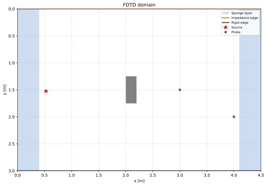
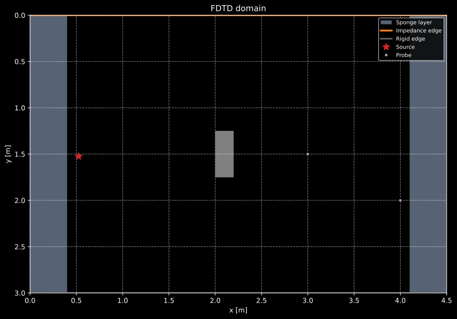
Everything the run will see, before it runs: the sponge layers eat the left and right boundaries, the top edge carries the anechoic $\rho c$ impedance, the untreated bottom stays rigid, and both probes sit clear of the obstacle and the sponges.

Show the code for this figure

import numpy as np
import matplotlib.pyplot as plt
from phonometry import simulation

mask = np.zeros((60, 90), dtype=bool)
mask[25:35, 40:44] = True
sim = simulation.FDTD2D(343.0, 0.05, shape=(60, 90), sponge_width=8,
                        sponge_sides=("left", "right"),
                        edge_impedance={"top": 413.0}, obstacle_mask=mask)
sim.add_source(simulation.GaussianPulse(10, 30, width=1e-3))

# Check the domain before running it: nothing has been stepped yet.
sim.plot_geometry(probes=[(3.0, 1.5), (4.0, 2.0)])
plt.show()

Checks that a run is usable

plot_geometry catches a scene that was built wrongly. These six catch a run that was computed wrongly, and every one of them is a line or two:

1. The energy must not trend upward. FDTD2D.energy() returns the total field energy in joules per metre of depth. It rises while the source injects and then settles onto a plateau, fluctuating by about 1 % because pressure and velocity are half a time step apart; in a closed lossless domain the plateau is flat, and with a sponge or a damping map it decays. A total that climbs after the source is off is energy being created, and the run is not usable however plausible the snapshot looks.
2. np.isfinite(sim.p).all() catches a blow-up before it silently poisons an FFT: once a single cell is inf, every spectrum taken from that record is nan and the plot is empty rather than wrong-looking.
3. No probe inside a sponge, an obstacle or a source cell. All three read something that is not the field: an obstacle cell holds exactly 0.0 for the whole run, a sponge cell reads the attenuated field on its way out, and a soft-source cell reads mostly the injection — on the barrier scene of section 5, a probe on the source cell peaks 6.7 times higher than probe A, 0.4 m away, and a probe inside the barrier reads exactly 0.0 for the whole run.
4. Apply the ten-cell rule with the smallest sound speed in the map, at the highest frequency the analysis will actually use — not with the air value, and not with the highest frequency the source happens to excite (section 3 sizes both).
5. Rerun at half the cell size and confirm the answer moves by less than the tolerance your claim needs. The scheme is second order, so a dispersion-limited quantity should move about four times less at half the spacing; a quantity that moves by the same amount again is limited by something else — the staircasing above, or the length of the record.
6. For a scene meant to be anechoic, run it once with the scatterer removed and check that the residual sits below the level you intend to report. That subtraction is exactly what ContourPhasors.subtract() automates in section 4, and what the in-situ absorption measurement of ISO 13472-1 does on a real road.

A three-row rigid-walled domain is a plane-wave tube, and with the per-cell damping map a porous sample becomes an equivalent fluid, which turns the solver itself into a measurable specimen: the impedance-tube guide runs the ISO 10534-2 and ASTM E2611 measurements virtually on exactly that domain, animations included, and recovers the analytic absorption and transmission loss of the modelled sample through the library’s own reduction chains (the tests/simulation cross-checks run this on every commit).

3. Sizing a run

Section 6 derives the one rule most FDTD texts give — ten cells per shortest wavelength — and it decides only $\Delta x$. Four more numbers decide whether a run says anything at all: the source bandwidth, the run duration, the sponge thickness, and, for a steady-state measurement, the transient you throw away before the DFT window you keep. Each of them has a rule, and each of them fails quietly when it is wrong.

Source bandwidth. A GaussianPulse of half-width width is $s(t)=A{e}^{-((t-t_0)/\text{width}{)}^2}$, whose magnitude spectrum is $e^{-(\pi f\text{width}{)}^2}$: it is 20 dB down at $f=0.483/\text{width}$ and 40 dB down at $0.683/\text{width}$. Work in the reader’s direction — choose $f_{\text{max}}$, take $\Delta x$ from it, then take $\text{width}\ge 0.5/f_{\text{max}}$ and the pulse is at least 20 dB down where the grid stops resolving. Equivalently, in terms of the grid, $\text{width}\ge 4.83\Delta x/c_{\text{min}}$, which at $\Delta x=1$ cm in air is $1.4\times 10^{-4}$ s — and is why the examples here use $3\times 10^{-4}$ s, exciting to about 1.6 kHz inside the 3.4 kHz the grid resolves. Energy above $f_{\text{max}}$ is not an error in itself; it simply travels at the wrong speed and comes back as a ripple tail behind the pulse. The rigid-box run of section 6 reads a mode at 299 Hz on a grid whose ten-cell limit is 1.7 kHz, so its narrower $2\times 10^{-4}$ s pulse costs it nothing. For a single-frequency study CWSource sidesteps the question entirely.

Duration. Three things set it, and the largest wins. Geometry: at minimum the domain crossing time $\sqrt{L_x^2+L_y^2}/c$, plus one round trip to the reflector for every echo that matters. Decay: long enough for the feature to be visible above what is still ringing. Spectrum: a probe FFT resolves $1/T$, so separating two modes 3 Hz apart takes a third of a second of record however fine the grid — which is exactly why the room-mode run below is 0.35 s long and the barrier run is 9 ms.

Sponge thickness. The layer ramps an absorption rate $\sigma$ quadratically from zero at its inner face to a peak at the outer edge. Because $\sigma$ decays pressure and velocity together, the characteristic impedance inside it stays $\rho c$ and a uniform lossy region would not reflect at all; everything that comes back is reflected by the gradient. That makes the rule a rule in cells, not in wavelengths, and it is worth seeing the measurement, taken at normal incidence on a plane-wave duct:

sponge_width	5	10	20	40	60
echo/incident at 1 kHz	−36 dB	−49 dB	−62 dB	−76 dB	−85 dB
echo/incident at 125 Hz	—	—	−61 dB	—	—

A 20-cell layer returns −61 dB at 125 Hz, where it is 0.07 wavelengths thick, and −64 dB at 2 kHz, where it is 1.2 wavelengths thick: the residual is flat within 3 dB over a 16:1 frequency range. Twenty cells is a good floor, forty is generous. sponge_reflection (default $10^{-4}$) sets the round-trip amplitude the ramp is designed for, and it is not a promise: at 20 cells the measured residual is −51 dB for $10^{-2}$, −62 dB for $10^{-4}$ and −59 dB for $10^{-6}$, because a more aggressive target makes the ramp steeper and the steeper ramp reflects more. The default is close to the optimum, and the way to buy more is thickness.

Two things the sponge does not do. First, it is far weaker at oblique and grazing incidence, where a wave running along the layer crosses very few cells of the ramp per wavelength travelled. Take the same 20-cell layer, put a pulse source 1 m above it, and measure what the layer adds to a probe at the same height by re-running with the layer 5 m away and subtracting: the addition is −30 dB relative to the direct arrival at 27° from the normal, −18 dB at 45°, −10 dB at 60° and −3 dB at 80°, against the −62 dB the same layer gives at normal incidence. A long shallow domain lined with sponges is therefore a duct, not a free field. The honest test is the one just described: move the boundary further out and confirm the probe trace does not change. Second, the sponge is not a place to stand — probes, sources and obstacles all belong clear of the layer (check 3 above).

Transient and window. A steady-state measurement runs in two parts: fill the domain, call probe.reset(), then integrate over an exact number of source periods. The transient to discard is the domain fill time $\sqrt{L_x^2+L_y^2}/c$, plus one traverse for each reflection that still matters, plus the source onset (ramp_cycles / frequency, three periods by default), plus the ring-up of any resonant geometry — roughly $Q$ periods, which is the whole reason the metadiffuser run below waits 8 ms where the bare monopole waits 4.5 ms: its necks and cavities are resonators and they have to fill. The window that follows should span an integer number of source periods so the on-the-fly DFT sees no truncation; ten periods is plenty.

In one line: $\Delta x$ from $f_{\text{max}}$ and $c_{\text{min}}$, $\Delta t$ from the Courant number and $c_{\text{max}}$, width from $\Delta x$, the sponge from the cell budget, the duration from the geometry and the spectral resolution, the transient from the domain and its resonances, and the window from the source period.

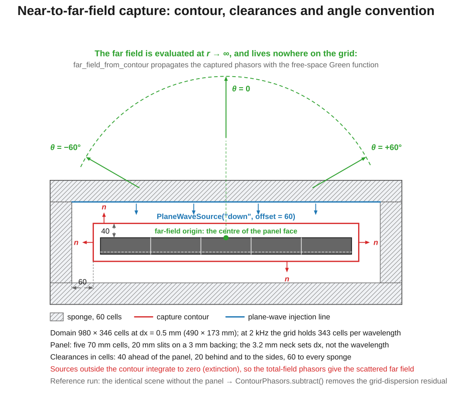
4. From the near field to the far field

A polar response or a diffusion coefficient is a far-field quantity, but an FDTD box ends a couple of wavelengths from the scatterer. The add_contour_probe / far_field_from_contour pair bridges that gap with the 2D Kirchhoff-Helmholtz integral: the probe folds the steady-state pressure and outward normal velocity on a closed rectangle of cell faces into complex accumulators (an on-the-fly DFT per point and frequency, so a continuous-wave run stores no time histories), and the integral propagates those phasors to infinity with the free-space Green function $-(j/4)H_0^{(2)}(kR)$ — the same construction full-wave FEM solvers use to report scattering patterns from near-field data. Two properties carry the scheme: the staggered grid already holds $v_n$ exactly on the contour faces, and any field whose sources lie outside the contour integrates to nothing (extinction), so the total-field phasors of a plane-wave scattering run transform directly into the scattered far field. In the discrete solver that cancellation leaves a grid-dispersion residual (below 0.01 dB on the scenes validated here); ContourPhasors.subtract() removes it with a no-scatterer reference run when that last fraction matters.

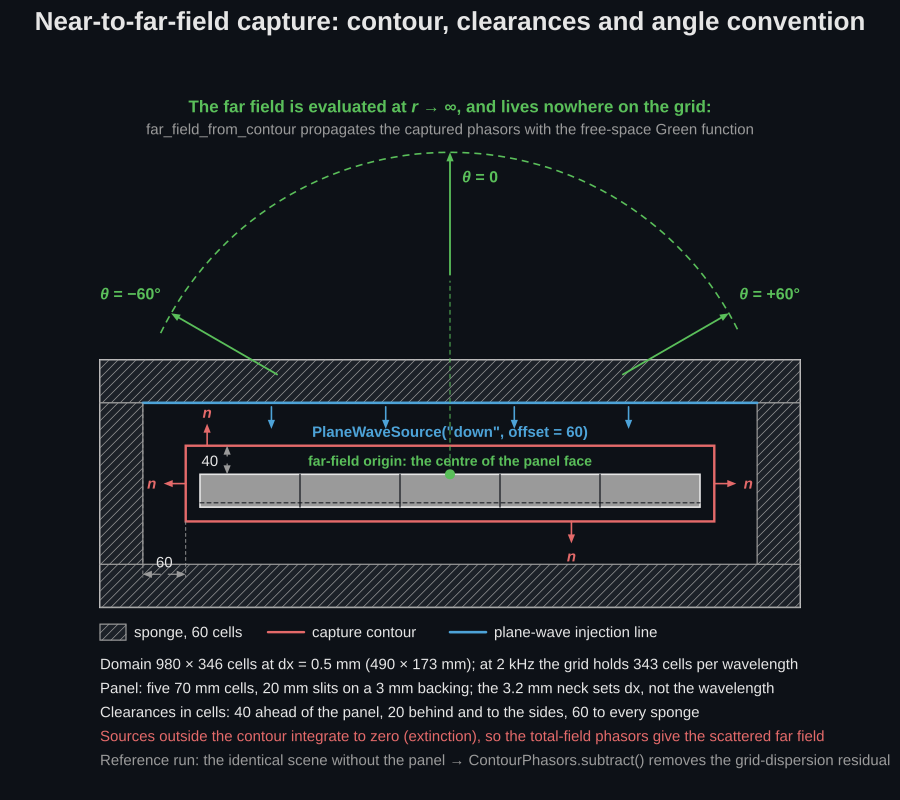
None of that is visible in the index arithmetic the snippets do, so here is the scene the metadiffuser run below actually builds, in true proportion.

import numpy as np
from phonometry import simulation

c0, dx, f0 = 343.0, 0.005, 2000.0
sim = simulation.FDTD2D(c0, dx, shape=(300, 300), sponge_width=40)
sim.add_source(simulation.CWSource(ix=150, iy=150, frequency=f0))
probe = sim.add_contour_probe(90, 210, 90, 210, frequencies=[f0])
sim.run(round(4.5e-3 / sim.dt))            # run the transient out
probe.reset()                              # then integrate the DFT window
sim.run(round(10.0 / f0 / sim.dt))
pattern = simulation.far_field_from_contour(
    probe.phasors(f0), np.arange(0.0, 360.0, 5.0),
    origin=(150.5 * dx, 150.5 * dx))
levels = 20 * np.log10(np.abs(pattern))
print(round(float(levels.max() - levels.min()), 2))   # 0.04 dB of ripple:
# a line source is omnidirectional, and its level matches the 2D
# free-space Green function to 0.11 dB

The analytic oracles behind those numbers run on every commit (tests/simulation): the reconstructed monopole pattern is flat within 0.05 dB and sits on the 2D Green-function level within 0.11 dB, an antiphase pair reproduces the two-source array factor within 0.4 % of the peak, and a contour that does not enclose the source transforms to less than 1 % of one that does. On top of them sit two meshed-panel cross-checks at 2 kHz: a quadratic-residue diffuser with wells to 27.4 cm, whose NTFF polar response tracks the Fraunhofer prediction of predict_diffuser_polar_response (pattern correlation 0.94, ISO 17497-2 directional diffusion coefficient within 0.08), and the deep subwavelength metadiffuser below.

The far-field chain is what finally closes the metadiffuser loop end to end: the Table-1 panel of the paper — every slit, neck and cavity meshed at 0.5 mm — driven to steady state by a plane wave, captured on a contour and transformed, against the metadiffuser_polar_response model (TMM + Fraunhofer) of the materials module. That is the library-side counterpart of the TMM-vs-FEM comparison the metadiffuser paper itself reports, small discrepancies included: the transfer-matrix model homogenises each 7 cm cell into one locally reacting reflection coefficient and ignores the evanescent coupling between neighbouring mouths, so the lobe structure agrees while individual nulls shift by a few degrees.

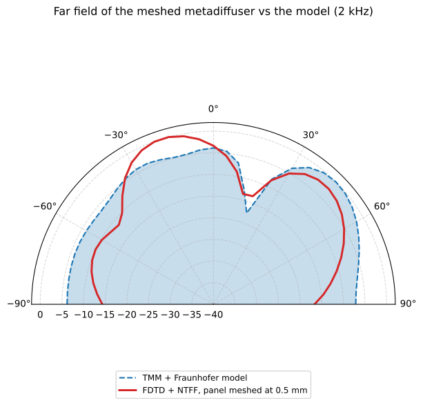
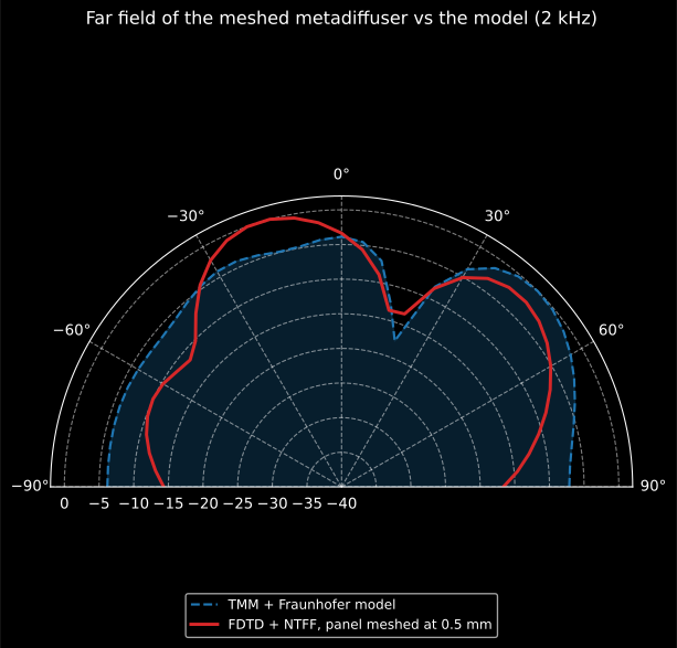
Two independent routes to the same far field: the meshed panel in a full-wave time-domain solver (solid) against the homogenised transfer-matrix chain (dashed). The lobes agree; the nulls, sensitive to the millimetre end corrections the TMM models analytically, shift by a few degrees.

Show the code for this figure

import numpy as np
import matplotlib.pyplot as plt
from phonometry import (HelmholtzResonator, MetadiffuserWell,
                        metadiffuser_polar_response, simulation)

c0, dx, f0, pitch = 343.0, 0.0005, 2000.0, 0.07
rows = [(14.7, 13.0, 16.4, 6.2, 9.0), (30.9, 9.1, 4.3, 3.5, 9.0),
        (30.9, 9.1, 4.3, 3.5, 9.0), (15.7, 13.3, 17.0, 6.3, 9.0),
        (20.3, 18.0, 20.7, 3.2, 9.0)]     # Table 1: h, l_n, l_c, w_n, w_c

# Mesh the real panel: a rigid slab with the slits, necks and cavities
# carved out at 0.5 mm (the 3.2 mm narrowest neck spans six cells).
sponge, gap, marg, front = 60, 60, 20, 40
face = round(5 * pitch / dx)
lat = marg + gap + sponge
r_face = sponge + gap + front
slab = round(0.023 / dx)                  # 2 cm panel + 3 mm back wall
mask = np.zeros((r_face + slab + marg + gap + sponge,
                 face + 2 * lat), dtype=bool)
mask[r_face:r_face + slab, lat:lat + face] = True
for n, (h, ln, lc, wn, wc) in enumerate(rows):
    xs = (n + 0.12) * pitch
    c0s, c1s = lat + round(xs / dx), lat + round((xs + h * 1e-3) / dx)
    mask[r_face:r_face + round(0.02 / dx), c0s:c1s] = False
    for m in range(2):                    # two resonators per slit
        ym, xn = (m + 0.5) * 0.01, xs + h * 1e-3
        r0 = r_face + round((ym - 0.5e-3 * wn) / dx)
        r1 = r_face + round((ym + 0.5e-3 * wn) / dx)
        mask[r0:r1, c1s:lat + round((xn + ln * 1e-3) / dx)] = False
        r0 = r_face + round((ym - 0.5e-3 * wc) / dx)
        r1 = r_face + round((ym + 0.5e-3 * wc) / dx)
        mask[r0:r1, lat + round((xn + ln * 1e-3) / dx):
             lat + round((xn + (ln + lc) * 1e-3) / dx)] = False

sim = simulation.FDTD2D(c0, dx, shape=mask.shape, sponge_width=sponge,
                        cfl=0.9, obstacle_mask=mask)   # 340 cells/lambda:
sim.add_source(simulation.PlaneWaveSource(           # dispersion negligible
    "down", simulation.CWSource(0, 0, f0).value, offset=sponge))
probe = sim.add_contour_probe(lat - marg, lat + face + marg - 1,
                              r_face - front, r_face + slab + marg - 1,
                              frequencies=[f0])
sim.run(round(8e-3 / sim.dt))             # transient (ramp + ring-up) out
probe.reset()
sim.run(round(10.0 / f0 / sim.dt))        # a 10-period DFT window (in steps)
angles = np.arange(-90.0, 90.1, 5.0)      # from the panel normal
pattern = simulation.far_field_from_contour(
    probe.phasors(f0), angles - 90.0,     # the normal points along -y
    origin=((lat + face / 2.0) * dx, r_face * dx))
levels = 20 * np.log10(np.abs(pattern) / np.abs(pattern).max())

wells = [MetadiffuserWell(h * 1e-3,
                          (HelmholtzResonator(ln * 1e-3, wn * 1e-3,
                                              lc * 1e-3, wc * 1e-3),) * 2)
         for h, ln, lc, wn, wc in rows]
model = metadiffuser_polar_response(f0, wells, depth=0.02, period=pitch,
                                    angles=angles, periods=1)
ax = model.plot(color="#1f77b4", marker="", linestyle="--",
                label="TMM + Fraunhofer model")
ax.plot(np.radians(angles), levels, color="#d62728", lw=2.2,
        label="FDTD + NTFF, panel meshed at 0.5 mm")
ax.set_ylim(-40.0, 2.0)
ax.legend(loc="lower center")
plt.show()

Why the nulls move is a question about geometry, and the two geometries are worth putting side by side: the panel the model prices, and the panel the solver steps on.

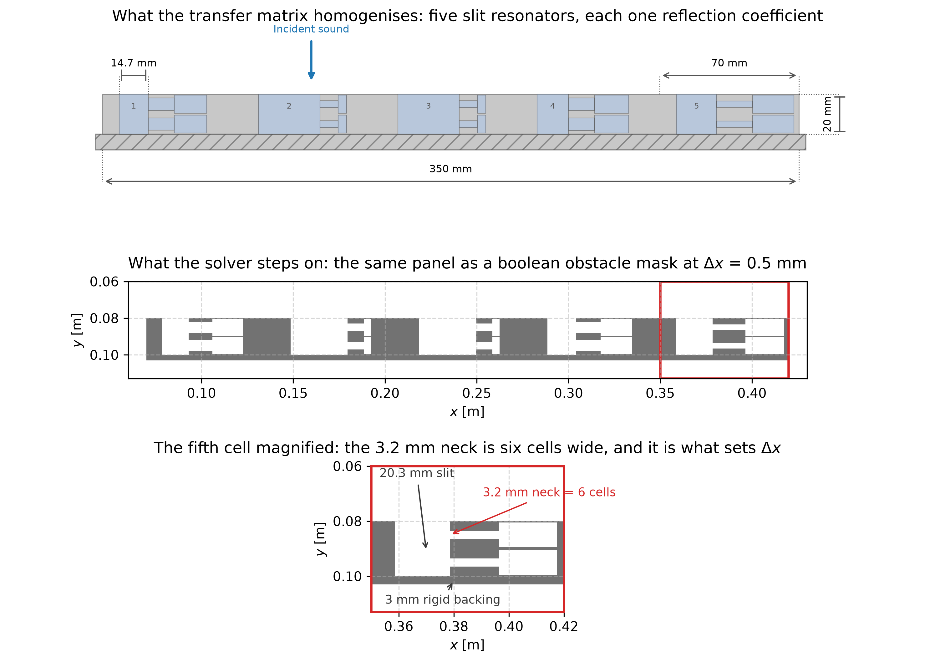
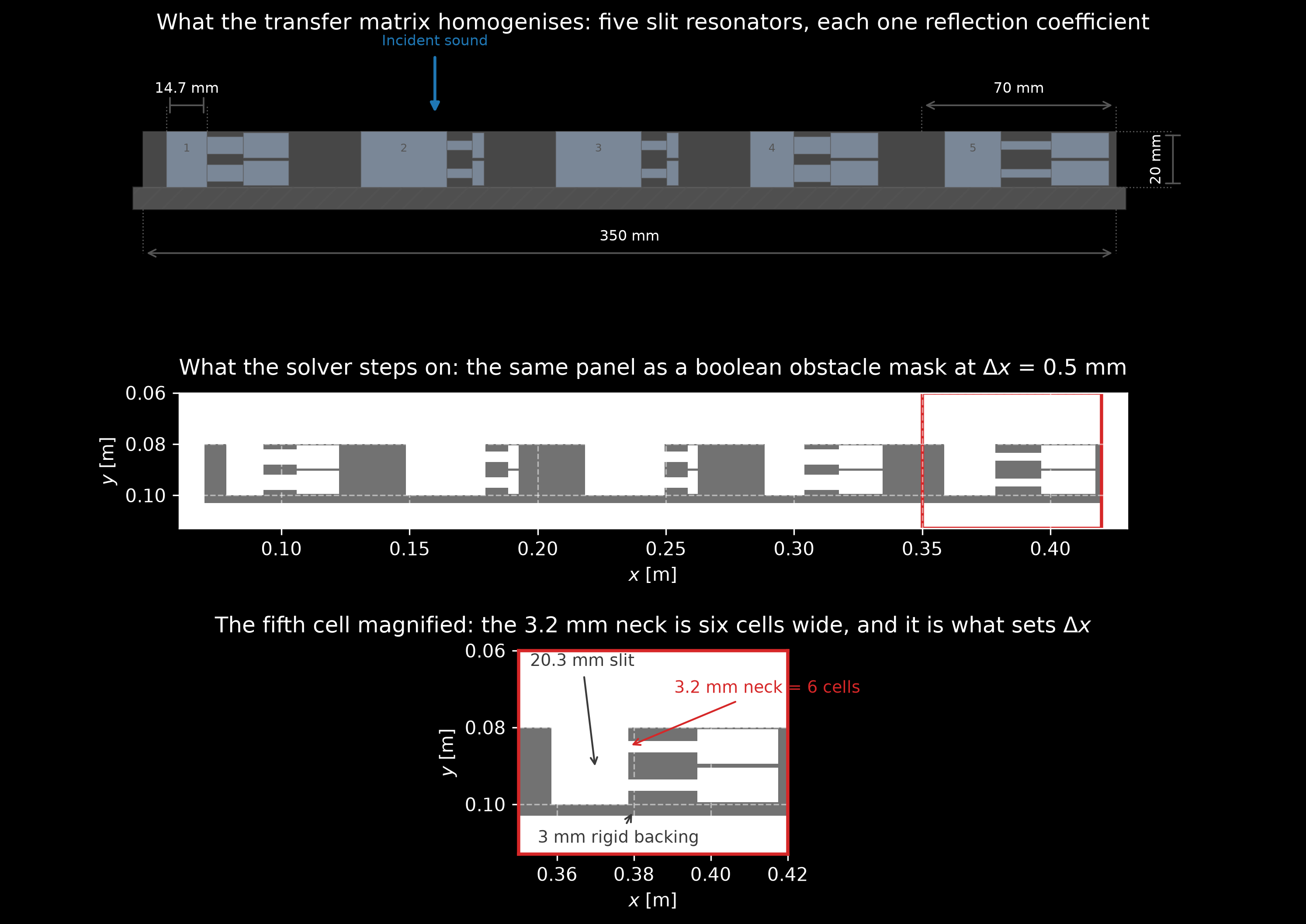
What the transfer matrix homogenises, against what the solver actually sees. The model turns each 70 mm cell into one locally reacting reflection coefficient; the mask keeps every slit, neck and cavity, and the evanescent coupling between neighbouring mouths comes for free because the mouths are really there. The narrowest neck is 3.2 mm — six cells at $\Delta x=0.5$ mm — and it, not the 17.2 cm wavelength, is what forces the grid. That difference is where the shifted nulls come from.

Show the code for this figure

# The model's view (top panel) is drawn by the library itself, from the same
# `wells` the block above built:
#     from phonometry.materials import plot_metadiffuser_panel_geometry
#     plot_metadiffuser_panel_geometry(wells, depth=0.02, period=0.07)

# The solver's view: the boolean mask the block above meshed, and one cell
# of it magnified.
fig, (ax_all, ax_cell) = plt.subplots(2, 1, figsize=(11, 6))
ax_all.imshow(mask[r_face - 40:r_face + slab + 20, lat - 20:lat + face + 20],
              cmap="Greys", interpolation="nearest")
cell = lat + round(4 * pitch / dx)
ax_cell.imshow(mask[r_face - 40:r_face + slab + 20,
                    cell:cell + round(pitch / dx)],
               cmap="Greys", interpolation="nearest")
plt.show()

5. When a wave simulation is worth it, and what 2D changes

FDTD earns its cost when the geometry drives the physics: diffraction around a barrier or through an opening, interference of direct and reflected paths, scattering from obstacles, modal behaviour of odd-shaped enclosures, refraction through a sound-speed gradient. One run captures all frequencies at once (a pulse excites the whole band; one FFT of a probe yields the spectrum), where a frequency-domain method needs one solve per frequency.

The barrier run below is the archetype. Nothing in its input says “diffraction”: the barrier is four columns of a boolean array, the source is a pulse, and the shadow-zone arrival is there anyway.

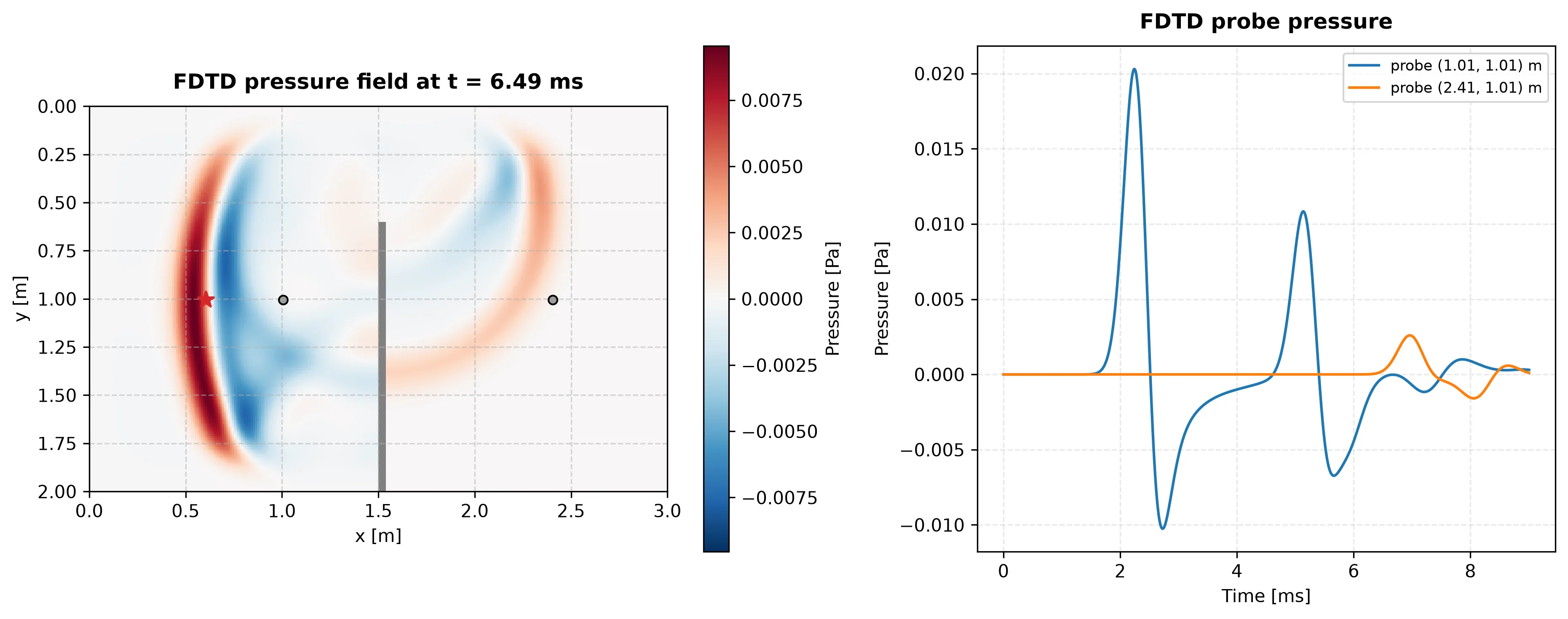
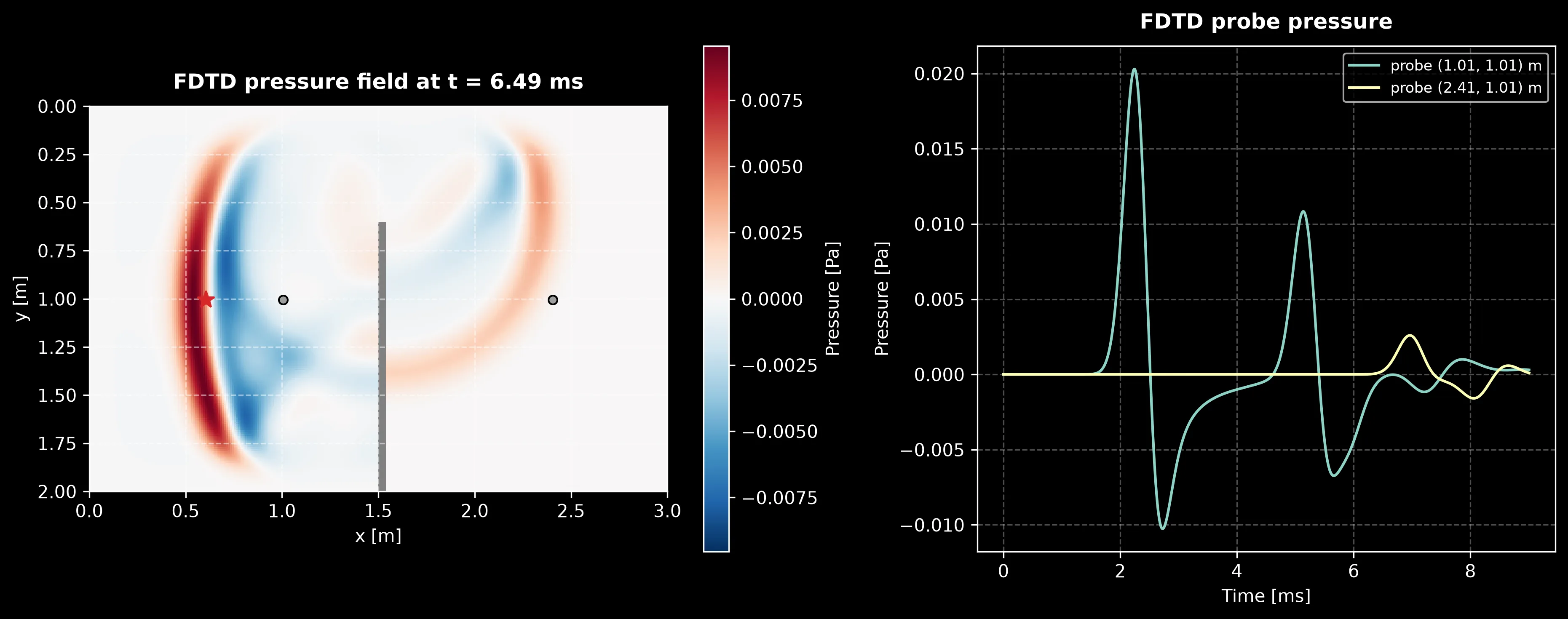
One run, two views. The snapshot (left, 6.5 ms in) holds the direct front, the reflection heading back past the source and the wave bending round the top edge of the barrier. In the traces (right), probe A on the line of sight records the direct pulse and then the barrier reflection, while probe B, in the shadow, records only the weaker and later arrival that came round the edge — an amplitude and a delay that no divergence-plus-attenuation formula produces on its own.

Show the code for this figure

import numpy as np
import matplotlib.pyplot as plt
from phonometry import simulation

# A 3.0 x 2.0 m free field (absorbing edges) with a thin rigid barrier:
# probe A sees the direct pulse plus the barrier reflection, probe B sits
# in the shadow and only receives the wave diffracted around the edge.
mask = np.zeros((200, 300), dtype=bool)
mask[60:, 150:154] = True
res = simulation.fdtd_simulation(
    343.0, 0.01, 9.0e-3, shape=(200, 300),
    sources=[simulation.GaussianPulse(ix=60, iy=100, width=3.0e-4)],
    probes=[(100, 100), (240, 100)],
    obstacle_mask=mask,
    boundaries="absorbing", absorbing_layer_cells=30,
    snapshot_every=75,
)

fig, (ax_f, ax_p) = plt.subplots(
    1, 2, figsize=(12.5, 5.0), gridspec_kw={"width_ratios": [1.25, 1.0]})
res.plot(kind="snapshot", frame=7, ax=ax_f)
res.plot(ax=ax_p)
plt.tight_layout()
plt.show()

Conversely, when a validated closed form exists (statistical reverberation, ISO 9613-2 outdoor attenuation, image sources in a rectangular room) it is thousands of times cheaper, and this solver is the cross-check and the demonstrator rather than the replacement. Section 6 shows one such cross-check reproducing the analytic room modes.

What a run costs. The work is cells × steps, and the single-threaded float64 stepping does of the order of $10^8$ cell-updates per second (measured: $8\times 10^7$ on the machine that renders these figures). The barrier scene above is 200 × 300 cells for 728 steps — $4.4\times 10^7$ updates, half a second. The metadiffuser scene of section 4 meshes at 0.5 mm into 346 × 980 cells and runs about 14 000 steps: $4.8\times 10^9$ updates, about a minute. The scaling between those two is the part worth remembering. In 2D, halving $\Delta x$ quadruples the cell count and, through the Courant condition, doubles the step count, so the work grows eightfold for a fourfold reduction in dispersion error. The ten-cell rule is therefore a floor to sit on, not a target to beat.

Memory follows the same arithmetic. The solver holds twelve float64 maps (pressure, the two velocity components, the sound speed, the density, the bulk modulus, the face densities and the decay factors) — about 96 bytes per cell, 113 with an obstacle mask, so the metadiffuser scene lives in about 39 MB. Stored snapshots are the knob nobody names: each one is another 8 bytes per cell, so snapshot_every=1 on that scene would ask for roughly 38 GB. Choose the cadence from the number of frames you actually want; the animations in this documentation use a few hundred. Probe histories cost one float per probe per step, which is nothing. The practical order of work is to size the grid from $f_{\text{max}}$, estimate the step count from the duration, and try the whole thing once at double the cell size to check the geometry and the probe placement before paying for the real run.

The domain is two-dimensional, and that changes the physics, not just the cost. A 2D point source is physically an infinite line source: its amplitude spreads cylindrically as $1/\sqrt{r}$ (3.0 dB per doubling of distance) instead of the spherical $1/r$ (6.0 dB) of a 3D point source, and the 2D impulse response trails a wake behind the wavefront instead of passing cleanly. Interference and diffraction patterns are faithful; absolute levels and decay rates are not those of a 3D room. Treat 2D runs as cross-sections and demonstrations, and validate any 3D-quantitative claim against a closed form or a 3D solver.

6. Numerical dispersion and accuracy

The discrete grid propagates each frequency at a slightly wrong speed: short wavelengths lag, so a sharp pulse develops a ripple tail and resonances shift slightly. This numerical dispersion is the discrete counterpart of Eq. 4.15; on the axes of a square grid the scheme’s dispersion relation is

$$\sin \left(\frac{\omega \Delta t}{2}\right)=\frac{c\Delta t}{\Delta x}\sin \left(\frac{k\Delta x}{2}\right),$$

with a leading-order relative frequency error of magnitude $(1-S^2)(k\Delta x{)}^2/24$ along the grid axes (the modelled frequency under-reads, so the signed error is negative), where $S=c\Delta t/\Delta x$ is the per-axis Courant number, which for square cells is the cfl value divided by $\sqrt{2}$ — the default cfl = 0.6 gives $S=0.424$ and $1-S^2=0.82$; the error is largest exactly on-axis and vanishes along the cell diagonal at the Courant limit $\mathrm{CN}=1$. The practical rule is to resolve at least 10 cells per shortest wavelength, $\Delta x\le c_{\text{min}}/(10f_{\text{max}})$ with the smallest sound speed of the domain: at exactly 10 cells the small-Courant bound $(k\Delta x{)}^2/24$ evaluates to about 1.6 %, reduced by the $1-S^2$ factor to about 1.4 % at the default cfl = 0.6 (in a heterogeneous domain the time step follows the fastest cells, so slower regions run at a lower local Courant number and sit nearer the 1.6 % bound), and every finer-resolved or off-axis component is more accurate. With $\Delta x=1$ cm the 10-cell point in air sits at roughly 3.4 kHz, and halving $\Delta x$ quarters the error (the scheme is second order, and the validation suite measures that observed order under grid refinement).

A pulse pays three times that. The error above is a phase speed error: it says a steady tone at wavenumber $k$ travels slightly slow. A pulse travels at the group speed, and differentiating the same dispersion relation gives $v_g/c=\cos \theta /\sqrt{1-S^2{\sin }^2\theta }$ with $\theta =k\Delta x/2$, whose expansion is $1-(1-S^2)(k\Delta x{)}^2/8$ — the same law with 8 in place of 24, so a wavepacket arrives three times later than the phase rule suggests. At 10 cells per wavelength and the default cfl that is 4.1 %, not 1.4 %. And because it is a speed error, it is paid per metre travelled: the same grid that is 4 % slow costs a centimetre over a metre and a metre over twenty-five.

The clip below measures both statements. One 500 Hz tone burst is launched down three plane tubes that are identical in every respect except $\Delta x$ — 137.2, 68.6 and 34.3 mm, which is 5, 10 and 20 cells per wavelength — and the exact continuous answer travels behind each trace in grey, so the numerical packet’s lag is a gap on screen rather than a number in a table.

A 500 Hz tone burst travels down three otherwise identical plane FDTD tubes meshed at 5, 10 and 20 cells per wavelength, with the exact continuous wave drawn behind each trace in grey. By the end of the run the coarse packet has fallen two wavelengths behind and grown a long ripple tail, the ten-cell packet lags by half a wavelength, and the twenty-cell packet still sits on the exact wave. Each panel prints its running lag in metres and, once the packet has crossed the 6.6 metre finish line, the crossing time and the measured speed deficit against the closed form. A side panel carries the phase-speed and group-speed error laws with the three grids marked.

Download the animation (WebM)

A 500 Hz tone burst travels down three otherwise identical plane FDTD tubes meshed at 5, 10 and 20 cells per wavelength, with the exact continuous wave drawn behind each trace in grey. By the end of the run the coarse packet has fallen two wavelengths behind and grown a long ripple tail, the ten-cell packet lags by half a wavelength, and the twenty-cell packet still sits on the exact wave. Each panel prints its running lag in metres and, once the packet has crossed the 6.6 metre finish line, the crossing time and the measured speed deficit against the closed form. A side panel carries the phase-speed and group-speed error laws with the three grids marked.

Download the animation (WebM)

Read three things off it. First, the lag grows: it is 0.14 m at 2.4 ms and 1.35 m by the end, because a speed error accumulates with distance. Second, the coarse tube grows a ripple tail behind the packet, not a reflection in front of it — the short components inside the burst travel slowest, so they arrive last. Third, the measured deficits are 17.2 %, 4.3 % and 1.1 % against 17.3 %, 4.3 % and 1.1 % from the closed form evaluated over the burst’s own spectrum, and the packets cross the finish line 3.3, 0.7 and 0.2 ms after the exact wave does. Halving $\Delta x$ quarters the error, in both laws and in the measurement.

The verification runs in both directions: the closed form pins the solver here, and once pinned the solver is what tests a closed form outside its own assumptions. A rigid-box run reproduces the analytic room modes.

import numpy as np
from phonometry import simulation

lx, ly, dx = 1.0, 0.7, 0.02
nx, ny = round(lx / dx), round(ly / dx)
res = simulation.fdtd_simulation(
    343.0, dx, 0.35, shape=(ny, nx),
    sources=[simulation.GaussianPulse(ix=7, iy=5, width=2.0e-4)],
    probes=[(nx - 4, ny - 3)],
)
p = res.pressures[0]
# Window the record (it ends with the undamped modes still ringing, and an
# abrupt truncation smears every peak) and zero-pad it eightfold, which
# interpolates the peak location without adding real resolution.
spec = np.abs(np.fft.rfft(p * np.hanning(p.size), n=8 * p.size))
freqs = np.fft.rfftfreq(8 * p.size, res.dt)
sel = (freqs > 250) & (freqs < 350)
print(round(0.5 * 343.0 * float(np.hypot(1 / lx, 1 / ly)), 1))  # 299.1  exact (1,1) mode
print(round(float(freqs[sel][np.argmax(spec[sel])]), 1))        # 298.9  measured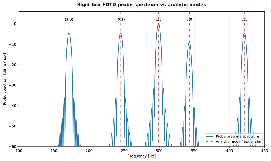

The probe spectrum of the rigid-box run peaks on the analytic mode frequencies $f=(c/2)\sqrt{(n_x/L_x{)}^2+(n_y/L_y{)}^2}$ (Kuttruff 6e, Ch. 3). The (1,1) peak lands 0.05 % low, and the bound above predicts 0.04 %, but read that agreement with care: at 0.35 s the raw bin spacing is 2.9 Hz and the eightfold padding interpolates to 0.36 Hz, so the 0.15 Hz shift is at the edge of what the record can resolve. Establishing the dispersion error properly means refining the grid, not reading one peak harder.

Show the code for this figure

import numpy as np
import matplotlib.pyplot as plt
from phonometry import simulation

lx, ly, dx, c = 1.0, 0.7, 0.02, 343.0
nx, ny = round(lx / dx), round(ly / dx)
res = simulation.fdtd_simulation(
    c, dx, 0.35, shape=(ny, nx),
    sources=[simulation.GaussianPulse(ix=7, iy=5, width=2.0e-4)],
    probes=[(nx - 4, ny - 3)],
)

# One line: the raw probe pressure history the spectrum is computed from.
res.plot()
plt.show()

# The mode check: probe spectrum against the analytic rigid-room modes.
p = res.pressures[0]
spec = np.abs(np.fft.rfft(p * np.hanning(p.size), n=8 * p.size))
freqs = np.fft.rfftfreq(8 * p.size, res.dt)
sel = (freqs >= 100) & (freqs <= 450)
fig, ax = plt.subplots()
ax.plot(freqs[sel], 20 * np.log10(spec[sel] / spec[sel].max()))
for mx, my in [(1, 0), (0, 1), (1, 1), (2, 0), (2, 1)]:
    ax.axvline(0.5 * c * np.hypot(mx / lx, my / ly), ls=":", color="tab:red")
ax.set(xlabel="Frequency [Hz]", ylabel="Probe spectrum [dB re max]",
       ylim=(-60, 6))
plt.show()

The tests pin the solver to analytic oracles the same way: box and duct eigenfrequencies, free-field arrival times and cylindrical decay, the rigid-wall image echo, the impedance reflection coefficient of section 2 and the dispersion relation itself.

The frozen FDTDResult carries the time axis, the per-probe pressure histories, the probe positions in metres, the grid metadata, the sources, the optional field snapshots with their times and the obstacle mask; its .plot() draws the probe histories, and .plot(kind="snapshot") renders one recorded field with the geometry overlaid.

The same staggered lattice extends beyond fluids: the companion elastic_fdtd_simulation integrates the P-SV velocity-stress system of Virieux (1986) on the same grid, adding shear waves, stress-imaging free surfaces with Rayleigh waves, and fluid-solid coupling with mode conversion, Scholte interface waves and immersed-plate transmission. That solver has its own guide, Elastic waves and fluid-solid coupling.

What this guide covers

• Covered

  The staggered pressure-velocity FDTD scheme of Attenborough & Van Renterghem, chapter 4: the governing equations (Eqs. 4.3-4.4), the leapfrog update (Eqs. 4.11-4.12), the Courant stability condition (Eqs. 4.13-4.14), the rigid boundary (Eq. 4.32) and the frequency-independent real-impedance boundary (Eqs. 4.33-4.35), exposed through fdtd_simulation/ FDTD2D with GaussianPulse, CWSource and SignalSource sources, pressure probes and a rasterised obstacle_mask, with damping as the only volumetric loss. Section 3 derives the four sizing rules the resolution rule does not cover — the source bandwidth, the run duration, the sponge thickness in cells, and the transient and DFT window of a steady-state measurement — and section 2 lists the six checks that say whether a run is usable. Validated against closed-form oracles: the rigid-room normal modes (Kuttruff §3), free-field arrival times and cylindrical 2D decay, the rigid-wall image echo, the impedance reflection coefficient and the dispersion relation of section 6, with the measured convergence order matching the scheme’s second-order design. The near-to-far-field chain of section 4: closed-contour phasor capture (add_contour_probe) and the 2D Kirchhoff-Helmholtz integral (far_field_from_contour, Williams ch. 8), validated against the exact monopole and dipole line-source fields, the extinction property, and the meshed QRD and metadiffuser panels against the library’s own Fraunhofer and TMM far-field models.

• Not covered

  Interior geometry is rigid by construction: only the four domain sides accept an impedance or a sponge, so an interior surface can be softened only by backing it with a lossy damping region, and that region is a frequency-independent equivalent fluid rather than a porous model. The solver is two-dimensional only: it models a line source in cross-section (cylindrical $1/\sqrt{r}$ spreading), not the spherical $1/r$ spreading of a 3D point source, so absolute levels and decay rates are not those of a 3D room. The open boundary is the quadratic-ramp absorbing layer described as “the simple precursor” of a true perfectly matched layer, not a PML itself. The governing equations assume a non-moving medium, so wind or flow advection is not modelled, and the only impedance boundary is the frequency-independent real one of Eqs. 4.33-4.35. Elastic media are not covered here: the P-SV companion solver, its free surfaces and its fluid-solid physics have their own guide, Elastic waves and fluid-solid coupling.

See also

• Elastic waves and fluid-solid coupling: the P-SV companion solver on the same staggered grid, with Rayleigh and Scholte waves, mode conversion and immersed plates.
• Conformance report: two of the closed-form validation anchors of section 6 run there.
• API reference: simulation.fdtd, simulation.ntff.

Quick answers

How do I choose the FDTD grid spacing?

Resolve at least 10 cells per shortest wavelength, $\Delta x\le c_{\text{min}}/(10f_{\text{max}})$, using the smallest sound speed in the domain. At exactly 10 cells the on-axis dispersion error bound is about 1.6 %, reduced to about 1.4 % at the default cfl = 0.6 (the per-axis Courant number is then $S=\mathrm{cfl}/\sqrt{2}=0.424$, so the $1-S^2$ factor is 0.82), and halving $\Delta x$ quarters the error (the scheme is second order). With $\Delta x=1$ cm the 10-cell point in air sits at roughly 3.4 kHz. That bound is a phase speed error; a pulse travels at the group speed and is three times slower still — 4.1 % at ten cells — and pays it per metre travelled, which section 6 measures on three grids.

How wide should the source pulse and the sponge be?

The GaussianPulse spectrum is $e^{-(\pi f\text{width}{)}^2}$, 20 dB down at $f=0.483/\text{width}$, so width $\ge 0.5/f_{\text{max}}$ keeps the injected energy inside the band the grid resolves. The sponge is a rule in cells, not in wavelengths: because its absorption rate acts on pressure and velocity together, the layer keeps a real $\rho c$ impedance and only its gradient reflects. Twenty cells return about −61 dB at normal incidence, flat within 3 dB from 125 Hz to 2 kHz; forty cells return about −76 dB. Tightening sponge_reflection past its 1e-4 default makes the ramp steeper and the residual worse. Section 3 works all of this, and the run duration and DFT window with it.

What Courant number keeps an FDTD simulation stable?

The explicit scheme is stable only while a wavefront crosses at most one cell per time step. With square cells the Courant number is $\mathrm{CN}=c\Delta t\sqrt{2}/\Delta x\le 1$ (Attenborough & Van Renterghem Eq. 4.13). fdtd_simulation derives the time step from the cfl parameter (that same $\mathrm{CN}$, default 0.6) and the largest sound speed in the map, rejecting values outside $(0,1)$. The per-axis Courant number of the dispersion relation above is a different number, $S=c\Delta t/\Delta x=\mathrm{CN}/\sqrt{2}$, which is 0.424 at the default.

Can I trust the absolute levels from a 2D FDTD run?

No. A 2D point source is physically an infinite line source: its amplitude spreads cylindrically as $1/\sqrt{r}$, 3.0 dB per doubling of distance, instead of the spherical $1/r$ (6.0 dB per doubling) of a 3D point source. Interference and diffraction patterns are faithful, but absolute levels and decay rates are not those of a 3D room; validate any 3D-quantitative claim against a closed form or a 3D solver.

References

• Attenborough, K., & Van Renterghem, T. (2021). Predicting outdoor sound (2nd ed.). CRC Press. https://doi.org/10.1201/9780429470806Chapter 4: the pressure-velocity FDTD reference model implemented here, from the governing equations (4.3-4.4) and the staggered leapfrog update (4.11-4.12) through the Courant condition (4.13-4.14), the phase-error analysis (4.15) and the rigid and finite-impedance boundary conditions (4.32-4.35). The module implements this textbook numerical method rather than a measurement standard, with this chapter as the citable reference formulation.
• Jiménez, N., Cox, T. J., Romero-García, V., & Groby, J.-P. (2017). Metadiffusers: Deep-subwavelength sound diffusers. Scientific Reports, 7, 5389. https://doi.org/10.1038/s41598-017-05710-5The meshed Table-1 panel and the near-to-far-field polar comparison of section 4 reproduce, with this solver, the TMM-vs-full-wave cross-check the paper reports.
• Kuttruff, H. (2016). Room acoustics (6th ed.). CRC Press. https://doi.org/10.1201/9781315372150Section 3.5 places time-domain wave-based methods among the numerical approaches to the wave equation in enclosures, and chapter 3 gives the rigid-room normal modes used as the analytic oracle.
• Williams, E. G. (1999). Fourier acoustics: Sound radiation and nearfield acoustical holography. Academic Press. https://doi.org/10.1016/B978-0-12-753960-7.X5000-1Chapter 8: the Helmholtz integral equation behind far_field_from_contour, with the outgoing free-space Green function and the far-field limit of the near-to-far-field transformation of section 4.