Impedance Tube

The impedance tube is the materials laboratory shrunk to a bench: a rigid duct a few centimetres across in which a loudspeaker drives a single plane wave against a small sample, and everything the sample does to that wave is read back from microphones in the tube wall. Because there is one wave and one angle, the tube recovers what a reverberation room cannot: the complex reflection factor and surface impedance at normal incidence, magnitude and phase, from a specimen the size of a coffee-cup lid. Three standards share the hardware and differ in method, and the library keeps their helpers separate and never mixes them: the standing-wave-ratio method of ISO 10534-1, the two-microphone transfer-function method of ISO 10534-2, and the four-microphone transfer-matrix method of ASTM E2611 that adds the transmission loss. The closing section runs the whole instrument, sample included, inside the FDTD solver and recovers the analytic answer through the same reduction chains.

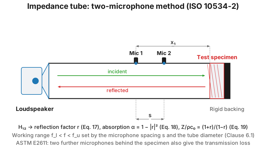
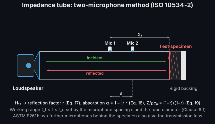
1. The working frequency range

Everything the tube reports (ISO 10534-2, Clause 4) assumes the field inside is a single plane wave, and the geometry sets both ends of the usable band. Above the cut-on of the first cross-sectional mode the field stops being planar: a circular tube of diameter $d$ needs $fd<0.58c_0$ (Eq. (2); $fd<0.50c_0$ for a rectangular tube, Eq. (3)). The microphone spacing $s$ must also stay clear of the half-wavelength singularity of the transfer-function method, $fs<0.45c_0$ (Eq. (4)). At the low end the opposite problem appears: a spacing much shorter than the wavelength leaves almost no phase difference between the microphones to measure, so the Clause 4.2 guideline keeps the spacing above 5 % of the wavelength:

$$\frac{c_0}{20s}<f<\min \left(0.58\frac{c_0}{d},0.45\frac{c_0}{s}\right).$$

No single tube covers the building-acoustics range. A 100 mm tube with a 100 mm spacing works from roughly 170 Hz to 1.5 kHz; reaching the 5 kHz bands takes a small tube (29 mm) with a close spacing, which in turn cannot see the low bands. Laboratories therefore pair a large and a small tube (or one tube with two spacings) and splice the spectra; the two must agree in the overlap bands, and a mismatch there points at the sample cut or mounting, not at the physics.

from phonometry import materials

# A 100 mm tube with 100 mm spacing, and a 29 mm tube with 20 mm spacing.
f_l, f_u = materials.plane_wave_frequency_range(0.100, 343.2, diameter=0.100)
print(round(f_l, 1), round(f_u, 1))     # 171.6 1544.4
f_l, f_u = materials.plane_wave_frequency_range(0.020, 343.2, diameter=0.029)
print(round(f_l, 1), round(f_u, 1))     # 858.0 6864.0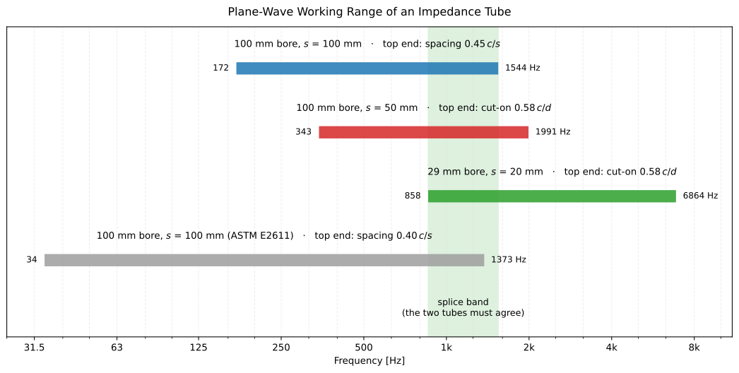

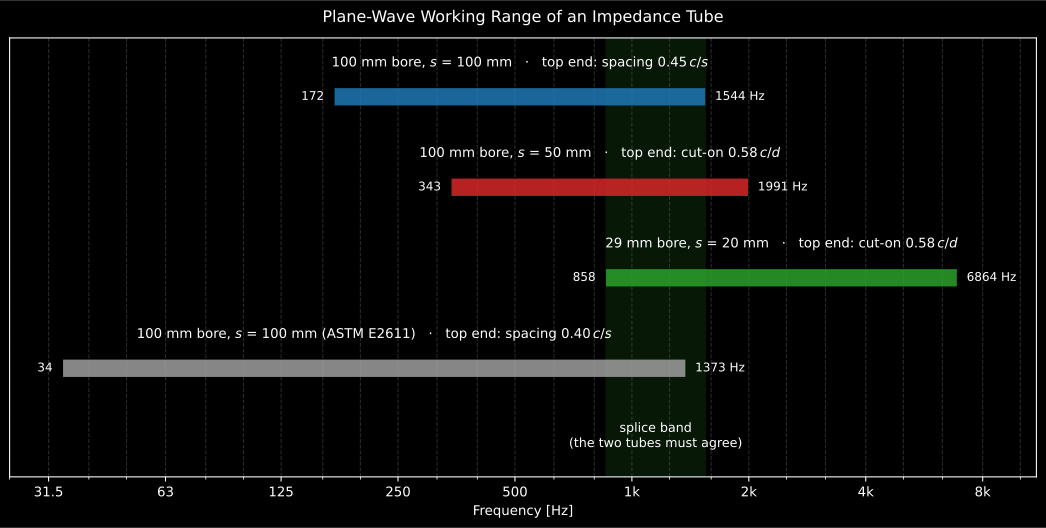
Which tube sees which bands. Each bar is a geometry, and each end is labelled with the constraint that binds it: the low end is always the $c_0/(20s)$ phase-resolution floor, while the top end is the cut-on $0.58c_0/d$ for a wide-spaced tube and the spacing singularity $0.45c_0/s$ once the microphones are far apart. The 100 mm tube with 100 mm spacing covers the 200 Hz to 1250 Hz one-third-octave bands and the 29 mm tube with 20 mm spacing the 1 kHz to 5 kHz bands, so the pair splices in the 1 kHz to 1.25 kHz overlap — and even together they do not reach the 100 Hz, 125 Hz and 160 Hz bands, which is why low-frequency absorption data come from the reverberation room and not from a tube. The ASTM bar is the same hardware under E2611’s constants: wider at the bottom (a 1 % of wavelength floor instead of 5 %) and narrower at the top (a $0.40c$ spacing bound instead of $0.45c$).

Show the code for this figure

for spacing, diameter in ((0.100, 0.100), (0.050, 0.100), (0.020, 0.029)):
    iso = materials.plane_wave_frequency_range(spacing, 343.2, diameter=diameter)
    astm = materials.plane_wave_frequency_range_astm(spacing, 343.2, diameter=diameter)
    print(f"{diameter * 1e3:.0f} mm bore, s = {spacing * 1e3:.0f} mm:",
          f"ISO {iso[0]:.0f}-{iso[1]:.0f} Hz, ASTM {astm[0]:.0f}-{astm[1]:.0f} Hz")

Those limits are easier to see on the hardware itself. plot_impedance_tube_geometry draws a tube to scale with its plane-wave band worked out, and a measured two_microphone_impedance result that was given its geometry (spacing, x1, diameter) redraws its own setup with result.plot_geometry().

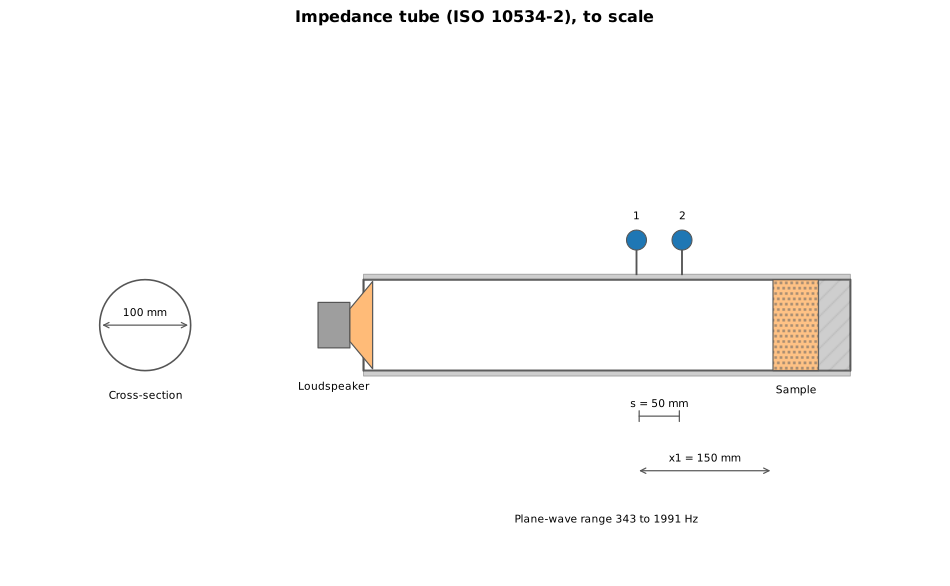
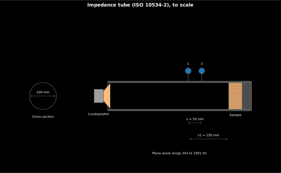
Everything the working-range inequalities talk about, in one to-scale side view: the 100 mm bore sets the 1991 Hz top end, the 50 mm spacing sets the 343 Hz bottom end, and the microphones sit at $s$ = 50 mm with the farther one $x_1$ = 150 mm from the specimen face.

Show the code for this figure

import matplotlib.pyplot as plt
from phonometry import materials

materials.plot_impedance_tube_geometry(spacing=0.05, x1=0.15, diameter=0.10)
plt.show()

# A measured result that retains its geometry draws its own tube:
#   res = materials.two_microphone_impedance(
#       h12, frequency=f, spacing=0.05, x1=0.15, diameter=0.10, ...)
#   res.plot_geometry()

1.1 Where the microphones may sit

The working range is set by $d$ and $s$; where along the tube the pair goes is a separate set of constraints, and Clause 4.3 fixes both ends of it.

Away from the source. The loudspeaker radiates cross-modes as well as the plane wave. Below the first cut-on they die out within about three tube diameters, so the nearest microphone is recommended to be at least three diameters from the source and shall in any case be no closer than one — 300 mm and 100 mm respectively on the 100 mm tube of the figure above.

Away from the specimen. The specimen distorts the field near its face too, and the minimum depends on what the specimen looks like: half a diameter for a non-structured sample, one diameter for a semi-laterally structured one, and two diameters for a strongly asymmetrical one. On a 100 mm tube that is 50 mm, 100 mm and 200 mm — so the $x_1$ = 150 mm of the figure above is comfortable for a plain porous sample, adequate for a perforated facing and too close for a strongly structured specimen such as a resonator array. Nothing enforces this: reflection_factor only rejects $x_1\le 0$, so an $x_1$ chosen by eye can sit inside the evanescent near field of a perforated sample and still return a perfectly plausible-looking spectrum.

How well the distances must be known. Fixed microphone positions to ±0.2 mm or better and traversing ones to ±0.5 mm (Clause 4.5); the reference plane’s position relative to microphone 1 reported to ±0.5 mm (Clause 7.1); and the microphone diameter under 20 % of the spacing, and small against $c_0/f_u$, so the capsule averages a negligible piece of the wave (Clause 4.4). The reference plane, $x=0$, is normally the specimen surface, but a profiled or laterally structured specimen has its reference plane placed some distance in front of it — and $x_1$ is measured to that plane, not to the sample holder.

The same helper covers square and rectangular tubes: pass shape="square" or shape="rectangular" and the Eq. (3) factor replaces the circular one, with $d$ the maximum side length. The four-microphone branch keeps its own limits in plane_wave_frequency_range_astm: ASTM E2611 retains the unrounded circular constant ($fd<0.586c$, 6.2.4.1), the same rectangular $fd<0.500c$ (6.2.5), a slightly stricter spacing bound $fs<0.40c$ (6.5.4) and a laxer low end at 1 % of the wavelength (6.2.3). Passing diameter= (and shape=) to two_microphone_impedance, wave_decomposition or the transfer_matrix_* solvers turns the matching check into an advisory warning, and for the Annex A attenuation estimate of a rectangular tube hydraulic_diameter(width, height) supplies the $4A/P$ diameter that tube_attenuation_constant expects.

The whole tube, sample included, can also be simulated: section 5 runs this exact measurement virtually inside the FDTD solver and recovers the analytic absorption of the modelled sample through the same reduction chain.

2. Standing-wave-ratio method (ISO 10534-1)

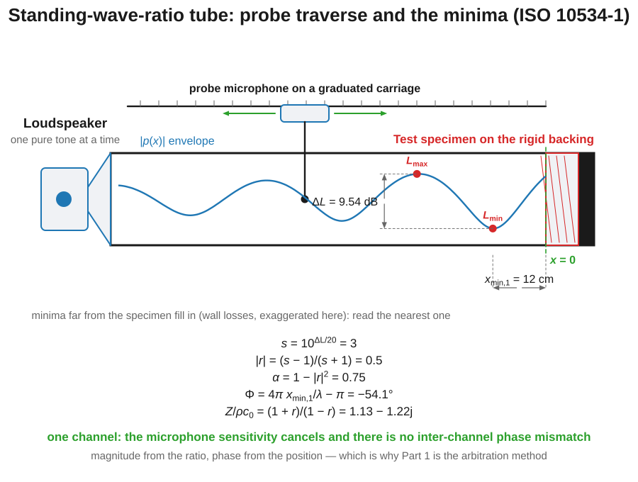
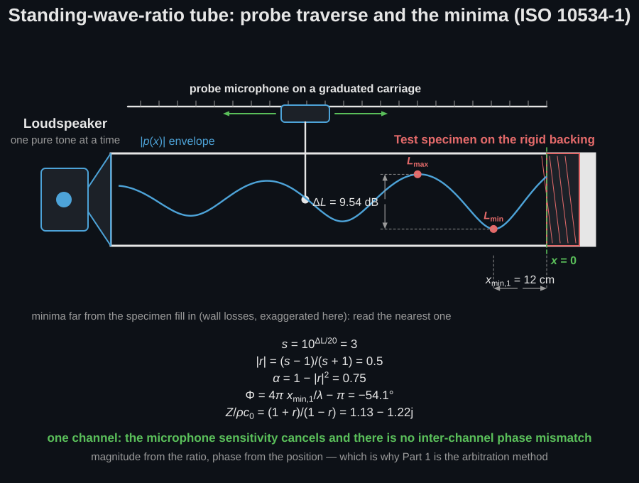
A probe traverses the standing wave and reads the level difference $\Delta L=L_{\text{max}}-L_{\text{min}}$ between a pressure maximum and the adjacent minimum. The standing-wave ratio — written $s$ in ISO 10534-1, the same letter Part 2 uses for the microphone spacing of section 1; the two never appear in the same equation, and the code keeps them apart as swr and spacing — follows in closed form together with the reflection magnitude and the absorption:

$$s=10^{\Delta L/20},|r|=\frac{s-1}{s+1},\alpha =1-|r{|}^2.$$

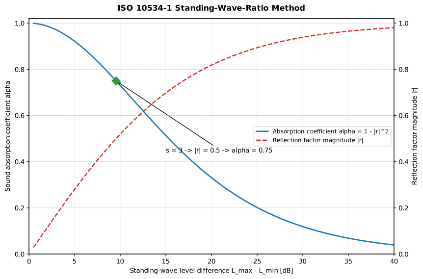
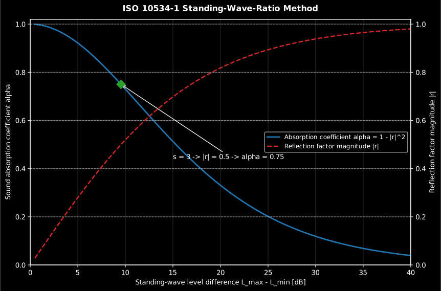
A small level difference means a near-perfect absorber; a level difference of 9.54 dB gives $s=3$, $|r|=0.5$ and $\alpha =0.75$.

Show the code for this figure

import matplotlib.pyplot as plt
import numpy as np
from phonometry import materials

level_diff = np.linspace(0.5, 40.0, 300)    # L_max - L_min [dB]
swr = materials.standing_wave_ratio_from_level(level_diff)
fig, ax = plt.subplots()
ax.plot(level_diff, materials.standing_wave_absorption(swr),
        label="Absorption coefficient alpha")
ax.plot(level_diff, materials.standing_wave_reflection_magnitude(swr), "--",
        label="Reflection factor magnitude |r|")
ax.set_xlabel("Standing-wave level difference L_max - L_min [dB]")
ax.set_ylabel("alpha, |r|")
ax.legend()
plt.show()

from phonometry import materials

s = float(materials.standing_wave_ratio_from_level(9.542))   # level difference [dB] -> SWR
print(round(s, 2))                                  # 3.0
print(round(float(materials.standing_wave_absorption(s)), 2)) # 0.75

The ratio method predates the FFT analyser and survives because it is self-contained. The apparatus is a probe microphone on a graduated carriage: a thin tube sliding along the axis, sampling the interior field point by point while the loudspeaker holds a single pure tone. At each frequency the operator (or the stepper motor) locates one pressure maximum and the adjacent minimum, reads the level difference, and moves on to the next tone. Slow, but there is nothing to calibrate against anything else: one microphone measures both levels, so its sensitivity cancels exactly, and there is no inter-channel phase mismatch because there is only one channel. That is why the standing-wave method remains the arbitration method when two transfer-function tubes disagree.

The closed forms above use only the level difference; the positions of the minima carry the rest of the information. With $x$ measured from the sample face towards the source, the interior field of a wave with reflection factor $r=|r|e^{j\Phi }$ is

$$p(x)=A\left(e^{jkx}+|r|e^{j\Phi }{e}^{-jkx}\right),|p{|}^2=A^2\left(1+|r{|}^2+2|r|\cos (2kx-\Phi )\right),$$

so pressure minima sit where the cosine is $-1$, at

$$2k{x}_{\min ,n}-\Phi =(2n-1)\pi ,\Phi =\frac{4\pi x_{\min ,1}}{\lambda }-\pi ,$$

with $x_{\min ,1}$ the minimum nearest the sample. A minimum a quarter wavelength from the face means $\Phi =0$ (a hard-backed sample at resonance); a minimum right at the face means $\Phi =-\pi$ (a rigid wall). Magnitude from the ratio, phase from the position: together they give the same complex $r$, and hence the same normalised impedance $Z/\rho c_0=(1+r)/(1-r)$, that the transfer-function method of section 3 computes from $H_{12}$ in one shot.

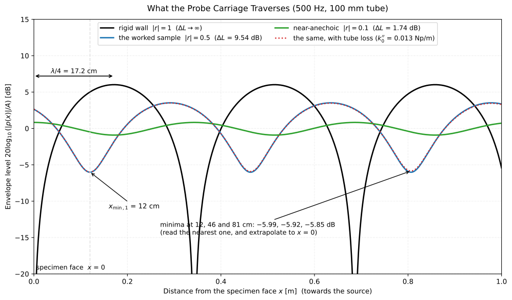
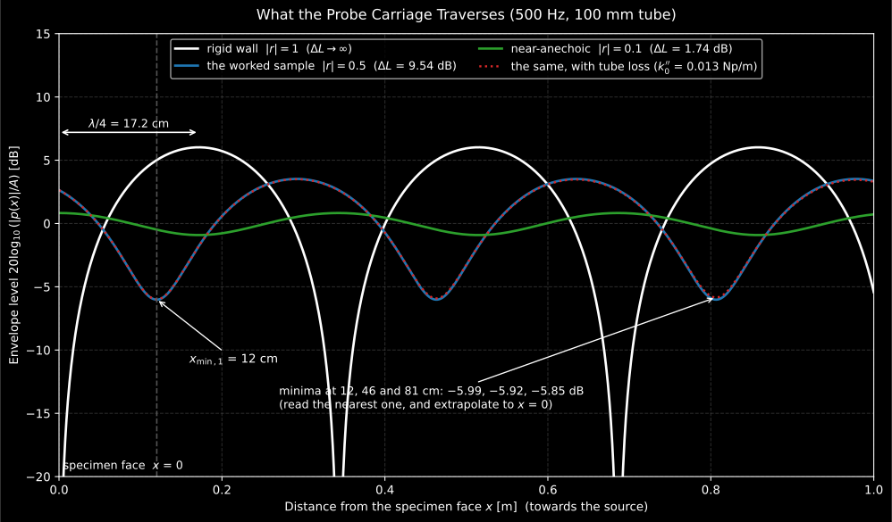
What the carriage actually traverses, drawn as the level the analyser shows at 500 Hz in a 100 mm tube. The rigid wall ($|r|=1$) has its minima on zero pressure and the first of them at the face, $\Phi =-\pi$; the worked sample ($|r|=0.5$) reads $\Delta L$ = 9.54 dB between the maximum and the adjacent minimum, the first of them at $x_{\min ,1}$ = 12 cm, and the quarter-wavelength ruler converts that distance into $\Phi =-54.1°$; the near-anechoic case ($|r|=0.1$) modulates by only 1.74 dB, which is why the method loses precision exactly where an absorber is good. The dotted curve is the same $|r|=0.5$ sample with the Eq. (A.18) tube attenuation: the further from the face, the more the reflected wave has decayed, so the notches fill in — the first three minima read −5.99, −5.92 and −5.85 dB. That drift is small here because Eq. (A.18) is a lower bound; ISO 10534-1’s approximate extrapolation (Annex A.2.1.4) is offered while the first-to-second minimum difference stays under 2 dB, and above that the attenuation has to be measured on the empty tube. Either way it is why the operator reads the minimum nearest the sample.

Show the code for this figure

# The interior field of section 2, for three reflection factors.
c0 = 343.2
x = np.linspace(0.0, 1.0, 800)
k = 2 * np.pi * 500.0 / c0
for magnitude, phi in ((1.0, -np.pi), (0.5, np.radians(-54.1)), (0.1, 0.0)):
    envelope = np.sqrt(1 + magnitude**2 + 2 * magnitude * np.cos(2 * k * x - phi))
    print(round(float(envelope.min()), 3), round(float(envelope.max()), 3))

# The attenuated variant uses the Eq. (A.18) lower-bound constant.
print(round(float(materials.tube_attenuation_constant(500.0, c0, 0.10)), 4))

Magnitude and position are the two halves of the reading, and the library takes them together: standing_wave_reflection(swr, x_min1, wavelength) returns the complex $r$ (Eqs. (17)-(23)) and standing_wave_normalized_impedance the ratio $Z/\rho c_0$ (Eqs. (24)-(26)). Both accept arrays, so a stepper-motor traverse that logs $(\Delta L,x_{\min ,1})$ per tone reduces to two calls:

import numpy as np
from phonometry import materials

# A three-tone traverse: the level difference and the first-minimum distance
# read at each frequency, which is all the method produces.
f = np.array([500.0, 1000.0, 2000.0])
c0 = 343.2
level_difference = np.array([9.542, 6.021, 3.522])   # L_max - L_min [dB]
x_min1 = np.array([0.120, 0.061, 0.030])             # first minimum [m]

swr = materials.standing_wave_ratio_from_level(level_difference)
lam = c0 / f
r = materials.standing_wave_reflection(swr, x_min1, lam)
z = materials.standing_wave_normalized_impedance(swr, x_min1, lam)
print(np.round(np.abs(r), 2))                  # [0.5  0.33 0.2 ]
print(np.round(np.degrees(np.angle(r)), 1))    # [-54.1 -52.  -54.1]
print(np.round(z, 2))                          # Z / rho c0

Two practical cautions from the standard’s own text. The minima far from the sample are shallower than the theory above says, because the travelling waves decay along the tube (viscous and thermal losses at the wall); ISO 10534-1 has the operator read the minimum nearest the sample and, for precision work, extrapolate the minimum levels to the sample face. And the method leans on the purity of the tone: any harmonic distortion from a hard-driven loudspeaker puts energy at frequencies whose minima sit elsewhere, partially filling the notch being measured, so the analyser must be narrowband around the drive frequency rather than a broadband level meter.

3. Transfer-function method (ISO 10534-2)

Two fixed microphones measure the complex transfer function $H_{12}$; from it the reflection factor at the sample face, the absorption and the normalised surface impedance follow (Eqs. (17)–(19)):

$$r=\frac{H_{12}-H_I}{H_R-H_{12}}{e}^{2j{k}_0{x}_1},\alpha =1-|r{|}^2,\frac{Z}{\rho c_0}=\frac{1+r}{1-r},$$

with $H_I=e^{-j{k}_{0}s}$, $H_R=e^{+j{k}_{0}s}$, microphone spacing $s$ (the Part 2 meaning of the letter again) and $x_1$ the distance from the reference plane to the farther microphone.

What an error in $x_1$ costs, and what it does not. $x_1$ enters only through $e^{2j{k}_0{x}_1}$, a pure phase rotation. It therefore leaves $|r|$ — and hence the absorption spectrum — completely untouched, while rotating the real and imaginary parts of the surface impedance. At 1.5 kHz in air a 2 mm error in $x_1$ rotates the reflection phase by about 6°, enough to move a flow resistivity fitted from that impedance noticeably. The practical consequences are two: measure $x_1$ to the reference plane — the specimen face, or the plane in front of a profiled specimen — rather than to the sample holder, since a specimen that does not sit where it was meant to moves $x_1$ with it; and read a healthy-looking $\alpha$ beside an implausible impedance (a negative real part, say) as an $x_1$ or a mismatch fault, not as a material result.

The incident and reflected waves travel inside a drawn impedance tube and their sum forms the standing-wave envelope; a rigid termination with deep envelope nodes is compared with a porous sample with shallow ones, sampled by the two flush wall microphones.

Download the animation (WebM)

The incident and reflected waves travel inside a drawn impedance tube and their sum forms the standing-wave envelope; a rigid termination with deep envelope nodes is compared with a porous sample with shallow ones, sampled by the two flush wall microphones.

Download the animation (WebM)

import numpy as np
from phonometry import materials

f = np.array([500.0, 1000.0, 1800.0])
x1, spacing, c0 = 0.12, 0.03, 343.2
k0 = materials.tube_wavenumber(f, c0)

# A measured transfer function H12 (here synthesised from r = 0.3 - 0.4j)
target = 0.3 - 0.4j
x2 = x1 - spacing
h12 = (np.exp(1j*k0*x2) + target*np.exp(-1j*k0*x2)) / \
      (np.exp(1j*k0*x1) + target*np.exp(-1j*k0*x1))

r = materials.reflection_factor(h12, spacing=spacing, x1=x1, wavenumber=k0)
print(np.round(materials.absorption_from_reflection(r), 3))     # [0.75 0.75 0.75]
print(np.round(materials.normalized_surface_impedance(r), 2))   # Z / rho c0
# [1.15-1.23j 1.15-1.23j 1.15-1.23j]
print(np.round(materials.normalized_surface_admittance(r), 2))  # its reciprocal,
# [0.41+0.43j 0.41+0.43j 0.41+0.43j]     what an impedance boundary condition wants

The high-level two_microphone_impedance wraps this chain and returns an ImpedanceTubeResult with absorption, reflection factor, surface impedance and normalised impedance, applying the plane-wave frequency-range check and optional tube attenuation. Its .plot() draws the absorption spectrum $\alpha (f)$ with the reflection-factor magnitude $|r|$ overlaid, and normalized_surface_admittance(r) gives the reciprocal quantity that a locally-reacting boundary condition — an FDTD or BEM wall, the library’s own solver — consumes.

3.1 Correcting the channel mismatch (Clause 7.5)

A channel is a microphone plus its preamplifier plus its analyser input, and no two are identical. ISO 10534-2 Clause 7.5 does not recommend correcting for that, it requires it: “one of the following procedures … shall be used”. Annex E.1.2 is blunter still — with two microphones the phase mismatch “is unavoidable and shall be compensated for” — and E.1.3 adds that the amplitudes should be within 0.3 dB of each other to begin with. The correction is a complex division applied exactly where $|r|$ is small and the phase of $H_{12}$ carries the whole answer, which is why the symptom of skipping it is frequency-dependent wander rather than an offset: the snippet below leaves a 0.5 dB / 1° mismatch uncorrected on a specimen whose true absorption is 0.75 and gets 0.73, 0.78 and 0.72 in three neighbouring bands. On a near-perfect absorber the same mismatch pushes the spectrum against the $\alpha =1$ ceiling, which is where the classic uncorrected-tube signature — an absorption just above 1 or just below 0 — comes from.

Both permitted procedures use the same measurement, made twice:

1. Place an absorptive specimen in the tube and measure $H_{12}^I$ in the standard configuration.
2. Physically interchange the two microphone cartridges, so that A takes the exact position B occupied and vice versa, without moving the cables on the preamplifier or the analyser. Measure $H_{12}^{II}$.
3. Form $H_c=\sqrt{H_{12}^I/H_{12}^{II}}$ (Eq. (10)) and divide the working transfer function by it.

The difference between the two procedures is only how often step 2 is done. Clause 7.5.1 repeats the swap for every specimen, which suits a small number of samples; Clause 7.5.2 determines $H_c$ once against a calibration specimen and keeps it for the whole series, which suits a production run — after which the microphones must stay where they are. The one-microphone technique of Annex B needs no correction at all, because there is only one channel: it buys that with measurement time, and it is the same argument that makes the standing-wave method of section 2 the arbitration method.

# A channel pair mismatched by 0.5 dB and 1 degree, and its removal. The two
# configurations differ by exactly that factor, which is what Eq. (10) recovers.
mismatch = 10 ** (0.5 / 20) * np.exp(1j * np.radians(1.0))
h12_i = h12 * mismatch            # standard configuration
h12_ii = h12 / mismatch           # microphones physically interchanged

hc = materials.mic_calibration_factor(h12_i, h12_ii)
print(round(float(np.abs(hc[0])), 4), round(float(np.degrees(np.angle(hc[0]))), 2))
# 1.0593 1.0 -- the mismatch itself, recovered
h12_corrected = materials.apply_mic_calibration(h12_i, hc)
print(float(np.abs(h12_corrected - h12).max()) < 1e-12)   # True

# What the uncorrected data would have claimed, on a sample of alpha = 0.75:
bad = materials.reflection_factor(h12_i, spacing=spacing, x1=x1, wavenumber=k0)
print(np.round(materials.absorption_from_reflection(bad), 3))   # [0.732 0.775 0.718]

3.2 The rest of the instrument

The reduction chain above is a few lines; the conditions that make its inputs trustworthy are most of ISO 10534-2. In the order they matter:

• The air, measured rather than assumed (Clause 7.2). $c_0$ and $\rho c_0$ are not constants of the method, they are readings. The tube air temperature must be measured and held to ±1 K with a transducer accurate to ±0.5 K, and the atmospheric pressure to ±0.5 kPa (Clause 4.12); Eq. (5) turns the first into $c_0$ and Eq. (7) the pair into $\rho$. The library exposes both: speed_of_sound_iso(temperature) takes kelvin, and air_density_iso(temperature, atmospheric_pressure) takes kelvin and kilopascals — the fiche snippet below feeds them straight into two_microphone_impedance instead of literals. Note that the ASTM E2611 helpers of section 4 take degrees Celsius, and the two are not interchangeable.
• Excitation (Clause 4.10, 7.3). A stationary signal with a flat spectral density over the range of interest: random, pseudo-random, periodic pseudo-random or chirp. The level must sit at least 10 dB above the background at every frequency of interest, and any frequency whose response is 60 dB below the maximum is rejected outright. The number of spectral averages follows from the accuracy wanted on $H_{12}$; a bandwidth-time product of 50 to 100 is the usual target (Annex E.2), and the record must be much longer than $2x_1/c_0$ or time aliasing corrupts it (Eq. (E.1)).
• Warm-up (Clause 5). At least 10 minutes of loudspeaker operation before the first measurement, so the tube air temperature has stopped drifting.
• The source end (Clauses 4.9, 4.11). The loudspeaker membrane covers at least two thirds of the tube cross-section, sits in an insulating box against airborne flanking to the microphones, and is elastically isolated from the tube — structure-borne excitation of the tube wall is a classic mimic of absorption. At least 200 mm of effective absorbent lining near the loudspeaker damps the air-column resonances.
• The specimen end (Clause 4.7). The back plate is rigid and tightly fixed, a metal plate of at least 20 mm being recommended, because it is the rigid termination most measurements rest on. A separate sample holder must match the tube bore to ±0.2 % and be sealed with vaseline rather than an elastic gasket.
• The analyser (Clause 4.8). More than 65 dB of dynamic range, and transfer-function errors from non-linearity, resolution, instability and temperature under 0.2 dB.

Everything the ISO 10534-2 report needs about the geometry is already in the fiche’s metadata block — tube diameter and shape, microphone spacing, mounting, temperature and pressure — so that block reads as a report checklist rather than decoration.

Tube attenuation, and when to switch it on. The plane wave in the tube is not lossless: viscous and thermal boundary layers at the wall attenuate the incident and the reflected wave over the distance $x_1$, and attenuation that is not accounted for is read as sample absorption. tube_attenuation_constant is the Eq. (A.18) estimate, $k_0^{\prime \prime }=1.94\times 10^{-2}\sqrt{f}/(c_{0}d)$, and its scaling says where it matters: it grows as $\sqrt{f}$ and falls as $1/d$, so a 29 mm tube suffers roughly three and a half times the loss of a 100 mm one at the same frequency, and moving the microphone pair closer to the specimen reduces it directly. It matters most for a near-perfect absorber, where the reflected wave is already weak. Two cautions come with it. Clause A.2.1.5 says plainly that this estimate ignores porous or dirty walls and any object in the tube, so it is a lower limit: a large discrepancy is a sign to clean or re-qualify the tube, not a number to trust. And the standard prefers the measured route — determine the attenuation from the empty tube at mid and upper frequencies (Eqs. (A.13)/(A.14), after every modification of the tube) and extrapolate downwards.

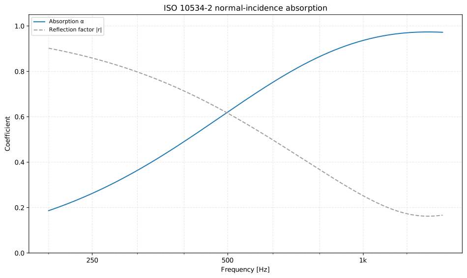
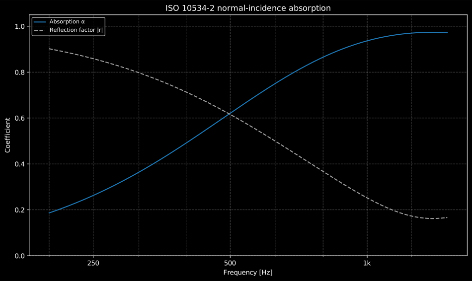
A 50 mm porous absorber measured over the working band of a 100 mm tube: the absorption climbs as the layer thickness grows against the wavelength, and $|r|$ falls as its mirror image ($\alpha =1-|r{|}^2$).

Show the code for this figure

import matplotlib.pyplot as plt
import numpy as np
from phonometry import materials

# A 50 mm porous absorber (Miki, sigma = 20 kPa s/m^2) in a 100 mm tube with
# 100 mm spacing (working band ~170 Hz to 1.5 kHz): the layer model supplies
# the true reflection factor, from which the transfer function H12 follows.
f = np.linspace(200.0, 1500.0, 260)
med = materials.miki(f, 20000.0)
layer = materials.layered_absorber(f, [materials.PorousLayer(0.05, med)])
spacing, x1, c0 = 0.10, 0.20, 343.2
k0 = materials.tube_wavenumber(f, c0)
x2 = x1 - spacing
r_true = layer.reflection
h12 = (np.exp(1j*k0*x2) + r_true*np.exp(-1j*k0*x2)) / \
      (np.exp(1j*k0*x1) + r_true*np.exp(-1j*k0*x1))
result = materials.two_microphone_impedance(
    h12, frequency=f, spacing=spacing, x1=x1, speed_of_sound=c0,
    characteristic_impedance=407.0, diameter=0.10,
)

# One line: alpha(f) with |r| overlaid.
result.plot()
plt.show()

# By hand, from the result's fields:
fig, ax = plt.subplots()
ax.plot(f, result.absorption, label="Absorption alpha")
ax.plot(f, np.abs(result.reflection), "--", label="Reflection factor |r|")
ax.set_xlabel("Frequency [Hz]")
ax.set_ylabel("Coefficient")
ax.legend()
plt.show()

ISO 10534-2 report (.report())

ImpedanceTubeResult.report(path) renders a one-page PDF fiche laid out like an accredited normal-incidence impedance-tube test report (ISO 10534-2:2001): a standard-basis line, a metadata header block, the per-frequency table (the absorption coefficient $\alpha$ and the real and imaginary parts of the normalised surface impedance $z=Z/\rho c_0$) beside the $\alpha (f)$ curve (the result’s own .plot(), on a continuous logarithmic frequency axis), a boxed characterisation headline and a footer with the fixed disclaimer. ISO 10534-2 is a characterisation, so the fiche carries no pass/fail verdict and no single-number rating; the normal-incidence coefficient is not comparable to the random-incidence ${\alpha }_s$/${\alpha }_w$ of ISO 354 / ISO 11654. Setting verbose=True inserts the reflection-factor magnitude $|r|$ column.

It uses the same ReportMetadata container and rendering engine as the other fiches. The measured frequency range is taken from the result; the applicable descriptive and geometric ReportMetadata fields are client, manufacturer, specimen, tube_diameter, tube_shape, mic_spacing, mounting, test_room, test_date, temperature, pressure, measurement_standard, laboratory, operator, report_id and notes (tube_diameter and mic_spacing are given in metres and printed in millimetres). The requirement field is ignored (ISO 10534-2 has no verdict). Rendering needs reportlab and, for the figure the fiche embeds, matplotlib (pip install "phonometry[report,plot]"); only engine="reportlab" is supported. The fiche renders in English by default; pass language="es" for a Spanish fiche (translated fixed strings and a comma decimal separator).

The block below is the specimen of the fiche underneath it: a resistive facing of normalised flow resistance $\theta =1$ over an 86 mm rigidly-backed air cavity, whose surface impedance $z=\theta -\mathrm{j}\cot (k_{0}L)$ is known in closed form, so the printed $\alpha$ can be checked by hand: 1.00 at the 1 kHz quarter-wave resonance, where the matched screen gives $z=1$ and $r=0$; 0.80 at 500 Hz, where $k_{0}L=\pi /4$ and $z=1-\mathrm{j}$.

import numpy as np
from phonometry import materials, ReportMetadata

# 100 mm tube, s = 50 mm, far microphone at x1 = 100 mm, 20 degC / 101 kPa.
c0 = float(materials.speed_of_sound_iso(293.15))                    # 343.29 m/s
rho_c = materials.characteristic_impedance(
    float(materials.air_density_iso(293.15, 101.0)), c0)            # 405.6 Pa.s/m
diameter, spacing, x1 = 0.100, 0.050, 0.100
theta, cavity = 1.0, c0 / (4.0 * 1000.0)          # quarter-wave at 1 kHz: 86 mm
freqs = np.array([400, 500, 630, 800, 1000, 1250, 1600], dtype=float)

# The transfer function the tube would measure, synthesised from the known r.
k0 = materials.tube_wavenumber(freqs, c0)
z = theta - 1j / np.tan(2 * np.pi * freqs / c0 * cavity)
r_known = (z - 1.0) / (z + 1.0)
x2 = x1 - spacing
h12_fiche = (np.exp(1j*k0*x2) + r_known*np.exp(-1j*k0*x2)) / \
            (np.exp(1j*k0*x1) + r_known*np.exp(-1j*k0*x1))

fiche = materials.two_microphone_impedance(
    h12_fiche, frequency=freqs, spacing=spacing, x1=x1,
    speed_of_sound=c0, characteristic_impedance=rho_c, diameter=diameter,
)
print(np.round(fiche.absorption, 2))    # [0.68 0.8  0.9  0.97 1.   0.96 0.68]

fiche.report(
    "alpha_fiche.pdf",
    metadata=ReportMetadata(
        specimen="Resistive facing over an 86 mm rigidly-backed air cavity",
        tube_diameter=diameter,        # m (printed as 100 mm)
        mic_spacing=spacing,           # m (printed as 50 mm)
        measurement_standard="ISO 10534-2",
        laboratory="Phonometry Reference Laboratory",
    ),
)                       # normal-incidence alpha and impedance over the tube band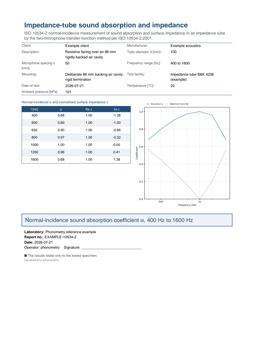

One-page normal-incidence impedance-tube fiche: a metadata header (client, specimen, tube diameter d, microphone spacing s, the measured frequency range, mounting, test facility, temperature and pressure), the per-frequency table of the absorption coefficient alpha and the real and imaginary parts of the normalised surface impedance z beside the alpha curve on a logarithmic frequency axis, and the boxed characterisation headline over the tested frequency range.

Download the report (PDF)

Normal-incidence impedance-tube fiche (ImpedanceTubeResult.report), the alpha spectrum with the surface impedance.

4. Transmission loss (ASTM E2611)

With four microphones (two upstream, two downstream of the sample) a two-load (or one-load) measurement recovers the sample’s transfer matrix, whose entries give the normal-incidence transmission loss, reflection and wavenumber:

$$\mathrm{TL}=20{\log }_{10}\left|\frac{T_{11}+T_{12}/\rho c+\rho c{T}_{21}+T_{22}}{2}\right|.$$

What a “load” is, and why there are two of them. A load is a downstream termination. The matrix has four unknowns, and one measurement of the four microphone transfer functions supplies only two independent equations, so the general method changes the termination and repeats the whole measurement: E2611 Clause 8.5.4.1 solves the two sets together (Eq. (22)). In practice the tube ends in a weakly anechoic termination — a wedge or pyramid of glass fibre about 30 cm long — and Clause 6.2.8 asks for it to be easily removable precisely so that an open or a blocked end can provide the second load. All four transfer functions of each load are referenced to one common channel, and each of them carries the same switched-configuration mismatch correction as section 3 (Clause 8.5.3): the four-microphone method does not escape that requirement, it multiplies it. The source end is sealed and isolated from the tube (Clause 6.4.2), as in Part 2.

The one-load method is not the general method with fewer steps. Clause 8.5.4.2 closes the system instead by assuming the specimen is geometrically symmetric — “presenting the same physical properties to the sound field on either side” — so that reciprocity gives $T_{11}=T_{22}$ and $T_{11}{T}_{22}-T_{12}{T}_{21}=1$ (Eq. (23)), and one termination, preferably the anechoic one, is enough. That holds for a homogeneous layer and fails for any asymmetric build-up: a facing on one side, a gradient density, a mounted membrane, a stack of unequal layers — which is most of what people actually put in a transmission tube. transfer_matrix_one_load does not and cannot detect the asymmetry: it warns about the plane-wave range and about an ill-conditioned denominator, and otherwise returns a plausible, wrong matrix, and with it a wrong transmission loss. The rule is simple: if the specimen has a front and a back, use two loads. If you believe it is symmetric, run both solvers and compare. None of this touches the hard-backed absorption route of section 3, which needs only the surface impedance.

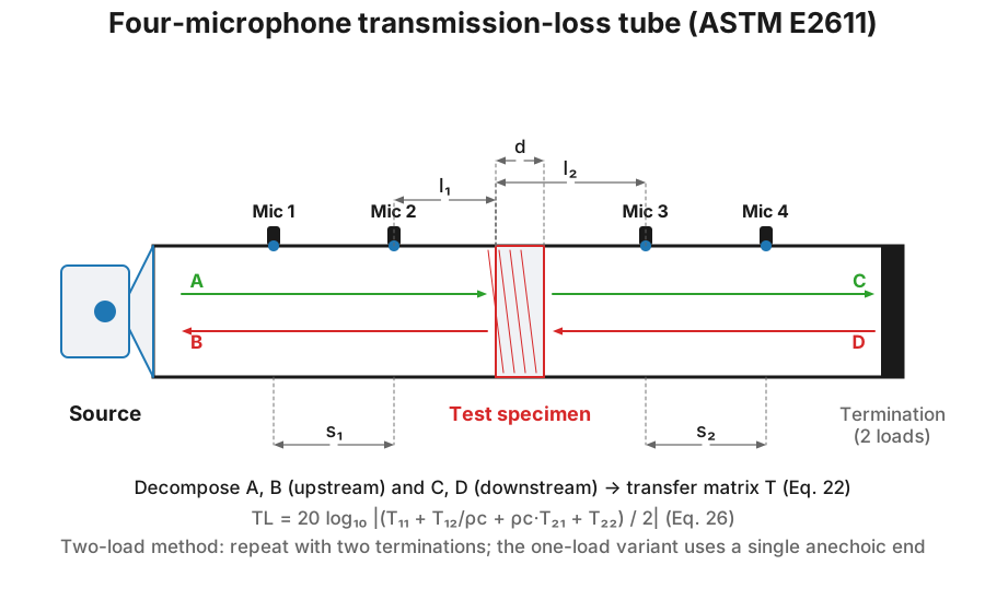
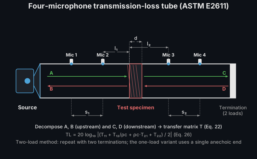
To scale it looks like this. A TransferMatrix recovered by the two-load or one-load solvers retains l1, s1, l2, s2 and the specimen thickness, so tm.plot_geometry() redraws the tube a measurement was taken in.

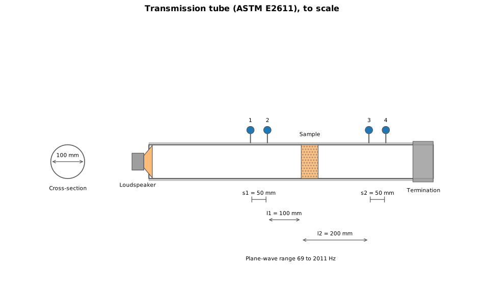
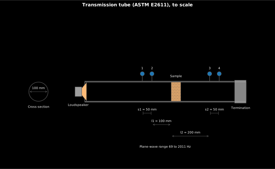
Where the four microphones of the transfer-matrix method actually sit around a 50 mm specimen in a 100 mm tube: $s_1=s_2$ = 50 mm, $l_1$ = 100 mm, $l_2$ = 200 mm, and the changeable termination that provides the second load. The ASTM working range for this geometry is 69 to 2011 Hz.

Show the code for this figure

import matplotlib.pyplot as plt
from phonometry import materials

materials.plot_transmission_tube_geometry(
    l1=0.10, s1=0.05, l2=0.20, s2=0.05, thickness=0.05, diameter=0.10,
)
plt.show()

# A TransferMatrix from transfer_matrix_two_load / _one_load retains its
# geometry, so tm.plot_geometry() redraws the tube it was measured in.

import numpy as np
from phonometry import materials

# An air layer is a known transfer matrix; TL = 0 dB (nothing is lost)
f = np.array([500.0, 1000.0, 2000.0])
k0 = 2*np.pi*f / 343.2
rho_c = 1.186 * 343.2
tm = materials.air_layer_transfer_matrix(thickness=0.05, wavenumber=k0,
                               characteristic_impedance=rho_c)
print(np.round(tm.transmission_loss(rho_c), 6))   # [0. 0. 0.]

transfer_matrix_two_load / transfer_matrix_one_load build the TransferMatrix from the four measured microphone transfer functions (H1, H2, H3, H4) of each load; its methods (transmission_loss, reflection_hard_backed, absorption_hard_backed, characteristic_impedance_material, material_wavenumber) then read off the ASTM E2611 quantities, and its .plot() draws the transmission loss with the hard-backed absorption overlaid (a matrix built by the solvers retains $\rho c$ and, when supplied, the frequency vector, so only a hand-built matrix needs them as arguments). The matrix does not have to come from a measurement: the multilayer solver exposes the chain matrix of any modelled stack in the same convention, so a predicted specimen can be read out exactly like a measured one.

import numpy as np
from phonometry import materials

# The chain matrix of a modelled 50 mm porous layer, read back through the
# ASTM E2611 machinery: TL and hard-backed absorption of the same specimen.
f = np.linspace(200.0, 1600.0, 300)
med = materials.miki(f, 20000.0)
layer = materials.layered_absorber(f, [materials.PorousLayer(0.05, med)])
chain = layer.transfer_matrix                       # shape (2, 2, len(f))
tm = materials.TransferMatrix(t11=chain[0, 0], t12=chain[0, 1],
                              t21=chain[1, 0], t22=chain[1, 1])
print(np.round(float(tm.transmission_loss(407.0)[-1]), 1))   # 9.7 dB at 1.6 kHz
tm.plot(f, 407.0)   # TL(f) with the hard-backed absorption overlaid

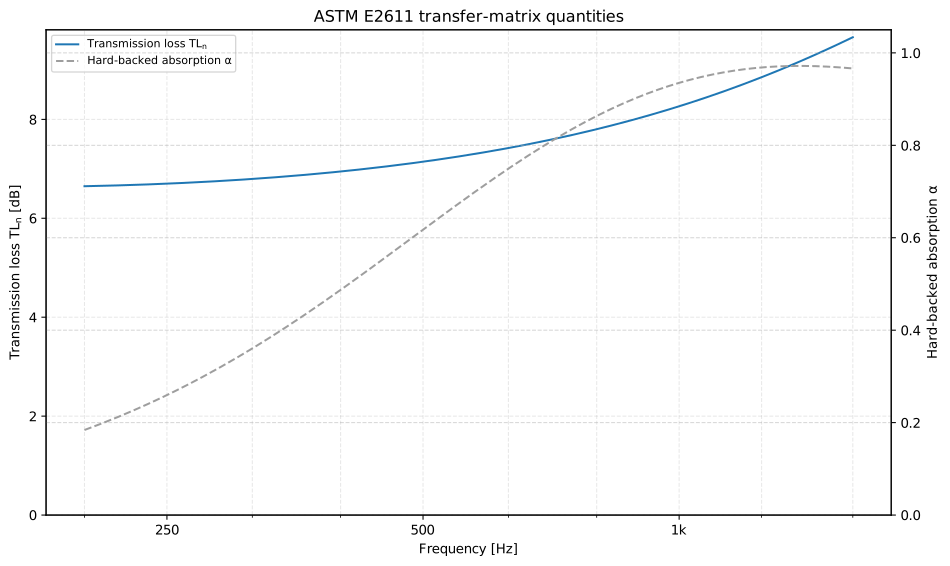
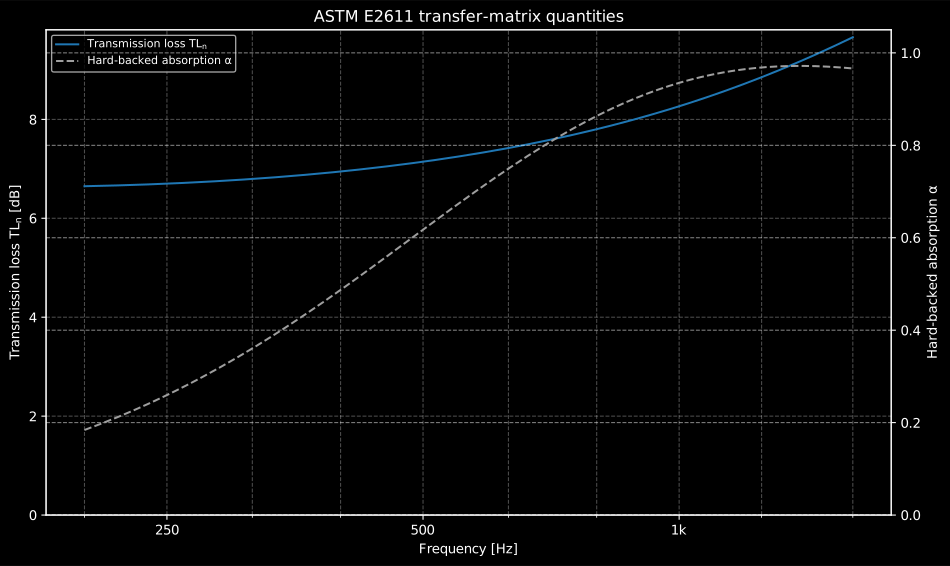
The same four-pole entries answer two different questions: how much sound the free-standing layer lets through (the transmission loss, Eq. (26)) and how much the rigidly-backed layer absorbs (Eq. (28)).

A tube TL is not a sound reduction index. The fiche of section 3 warns that the normal-incidence $\alpha$ is not the random-incidence ${\alpha }_s$; the same warning applies on the transmission side and is missed more often. What the tube measures is the transmission loss of a specimen a few centimetres across, for one plane wave at one angle, with the specimen edges clamped by the tube wall. What the sound reduction index $R$ is, is a diffuse-field quantity measured on a full-size element with its real mounting, and it carries the element’s own bending waves, its edge conditions and its coincidence dip — none of which exist inside a tube. Expect the normal-incidence value to sit above a field-incidence estimate for a mass-controlled layer, and expect the tube to miss the resonance and coincidence dips of a real panel entirely. Use the tube TL to compare materials and to fit and verify a transfer-matrix model; then predict the construction with the model, or with EN 12354, and never by carrying the tube number into a partition calculation.

Show the code for this figure

import matplotlib.pyplot as plt
import numpy as np
from phonometry import materials

f = np.linspace(200.0, 1600.0, 300)
med = materials.miki(f, 20000.0)
layer = materials.layered_absorber(f, [materials.PorousLayer(0.05, med)])
chain = layer.transfer_matrix                       # shape (2, 2, len(f))
tm = materials.TransferMatrix(t11=chain[0, 0], t12=chain[0, 1],
                              t21=chain[1, 0], t22=chain[1, 1])

# One line: TL(f) on the left axis, hard-backed absorption on the right.
tm.plot(f, 407.0)
plt.show()

# By hand, from the matrix methods:
fig, ax = plt.subplots()
ax.plot(f, tm.transmission_loss(407.0), label="Transmission loss TL_n")
twin = ax.twinx()
twin.plot(f, tm.absorption_hard_backed(407.0), "--", color="gray",
          label="Hard-backed absorption alpha")
ax.set_xlabel("Frequency [Hz]")
ax.set_ylabel("Transmission loss TL_n [dB]")
twin.set_ylabel("Hard-backed absorption alpha")
plt.show()

Mounting pitfalls

Most bad tube data are made at the sample holder, long before the signal processing. The recurring failures:

• Perimeter gaps. A specimen cut slightly undersize leaves an air sliver along the tube wall. Sound short-circuits around and behind the sample, and the gap itself resonates, so the measured absorption grows a spurious low-to-mid-frequency hump. Cut for a snug slide fit and seal the rim (a thin film of petroleum jelly is the classic remedy) without loading the front face.
• Compression. A specimen cut oversize and forced in is denser than the product it is supposed to represent: the flow resistivity rises, a limp frame is stiffened, and the absorption curve shifts and flattens. The result is repeatable and wrong.
• Hidden back cavity. If the specimen does not sit flush on the rigid backing, the unintended air layer acts as a quarter-wavelength cavity and moves the absorption peak down in frequency, flattering the material. Backing air gaps are perfectly legitimate mountings, but only when they are deliberate, dimensioned and reported with the result.
• Face not plane. A bulging, tilted or torn front face scatters into cross-sectional modes below the nominal cut-on and breaks the normal-incidence assumption the equations rest on. Cut with a sharp tool; do not tear fibrous materials to size.
• One specimen is not the material. Porous products are inhomogeneous at the scale of a tube sample. Measure several cuts and average; a spread between specimens is product variance worth reporting, not measurement noise to hide.

5. The virtual tube: the solver measured by the standards

A three-row rigid-walled domain of the 2D FDTD solver is a plane-wave tube, and with the per-cell damping map a porous sample becomes an equivalent fluid (density, speed and loss maps). That closes a remarkable loop: the FDTD probe histories can be reduced through the library’s own ISO 10534-2 and ASTM E2611 chains as if they were measurements, and the recovered spectra agree with the exact analytic answer for the same lossy layer to within 0.035 in absorption and 0.1 dB in transmission loss (the tests/simulation cross-checks run this on every commit).

import numpy as np
from phonometry.materials import two_microphone_impedance
from phonometry.simulation import FDTD2D

c0, rho0, dx = 343.0, 1.2, 0.005
nx, d_cells = 280, 20                     # 1.4 m tube, 10 cm sample
c = np.full((3, nx), c0); rho = np.full((3, nx), rho0)
sigma = np.zeros((3, nx))
c[:, -d_cells:] = 0.6 * c0                # the sample: slower,
rho[:, -d_cells:] = 3.0 * rho0            # denser and lossy
sigma[:, -d_cells:] = 600.0
sim = FDTD2D(c, dx, rho=rho, damping=sigma,
             edge_impedance={"left": rho0 * c0})   # anechoic source end
sim.add_plane_wave("right", center=0.35, width=0.05)
mics = (219, 229)                         # the ISO microphone pair
records = np.zeros((2, 9000))
for n in range(records.shape[1]):
    sim.step()
    records[:, n] = sim.p[1, mics]
spec = np.fft.rfft(records, axis=1)
freqs = np.fft.rfftfreq(records.shape[1], sim.dt)
band = (freqs > 300.0) & (freqs < 1200.0)
result = two_microphone_impedance(
    spec[1, band] / spec[0, band], frequency=freqs[band],
    spacing=0.05, x1=(nx - d_cells) * dx - (mics[0] + 0.5) * dx,
    speed_of_sound=c0, characteristic_impedance=rho0 * c0)
result.plot()   # the absorption the virtual tube "measured"

The two clips below run exactly this experiment. In the impedance tube a sustained plane tone builds the standing wave the two microphones read: against the rigid end the minima are deep, in front of the sample they stay shallow. In the transmission tube a carrier packet crosses an anechoic duct: the empty tube passes it unchanged, the lossy layer splits it into a reflection and an attenuated transmission that the four ASTM microphones resolve.

A loudspeaker drives a sustained 850 Hz plane tone into a 1.2 metre rigid-walled virtual impedance tube, drawn as the real instrument with its two flush microphones and rigid end plug. Against the rigid plug the standing-wave envelope grows deep minima, while a 10 cm lossy sample in front of the same plug leaves the minima shallow; the recovered absorption of 0.54 is annotated.

Download the animation (WebM)

A loudspeaker drives a sustained 850 Hz plane tone into a 1.2 metre rigid-walled virtual impedance tube, drawn as the real instrument with its two flush microphones and rigid end plug. Against the rigid plug the standing-wave envelope grows deep minima, while a 10 cm lossy sample in front of the same plug leaves the minima shallow; the recovered absorption of 0.54 is annotated.

Download the animation (WebM)

The loudspeaker end fires a carrier packet down a 1.6 metre rigid-walled virtual transmission tube drawn as the real instrument, with its four flush microphones and hatched anechoic termination. The empty tube passes the packet unchanged; a 10 cm lossy layer mid-tube splits it into a reflected train and an attenuated transmission, with the 3.1 dB transmission loss annotated.

Download the animation (WebM)

The loudspeaker end fires a carrier packet down a 1.6 metre rigid-walled virtual transmission tube drawn as the real instrument, with its four flush microphones and hatched anechoic termination. The empty tube passes the packet unchanged; a 10 cm lossy layer mid-tube splits it into a reflected train and an attenuated transmission, with the 3.1 dB transmission loss annotated.

Download the animation (WebM)

What this guide covers

• Covered

  The impedance-tube trio. The ISO 10534-1 standing-wave-ratio method (standing_wave_ratio_from_level, standing_wave_reflection_magnitude, standing_wave_absorption, and the position half of the reading in standing_wave_reflection and standing_wave_normalized_impedance). The ISO 10534-2 transfer-function method with its Clause 4 frequency-range check (two_microphone_impedance, plane_wave_frequency_range, reflection_factor, absorption_from_reflection, normalized_surface_impedance, normalized_surface_admittance, the Clause 7.2 air properties speed_of_sound_iso and air_density_iso, the Clause 7.5 mismatch pair mic_calibration_factor and apply_mic_calibration, and tube_attenuation_constant). The ASTM E2611 four-microphone transfer-matrix method (transfer_matrix_two_load, transfer_matrix_one_load, TransferMatrix, plane_wave_frequency_range_astm, hydraulic_diameter), with the to-scale geometry drawings of both tubes. The virtual FDTD tubes of section 5, whose recovered spectra are cross-checked against the analytic answer on every commit.

• Not covered

  Two editions cited only as later revisions are not implemented: ISO 10534-2:2023 (the code follows the 1998/2001 transfer-function method) and ASTM E2611-24 (the code follows E2611-19). ISO 10534-1:1996 is implemented as its European adoption BS EN ISO 10534-1:2001, not read directly from the 1996 ISO text; its probe-traverse refinements (extrapolating the minimum levels to the sample face, probe-body corrections) are described in section 2 but not automated. Neither are the equipment and procedure clauses of sections 1.1 and 3.2: the near-field distances of Clause 4.3, the position tolerances of Clause 4.5, the signal-to-noise floor of Clause 7.3 and the warm-up of Clause 5 are stated for the operator, and nothing in the library checks that any of them was met. tube_attenuation_constant implements only the Eq. (A.18) estimate, which the standard itself calls a lower limit; the measured determination of Eqs. (A.13)/(A.14) from the empty tube is not implemented. The random-incidence ${\alpha }_s$ of the reverberation room is a different quantity with its own guide: Sound Absorption Measurement and Rating.

See also

• Sound Absorption Measurement and Rating: the random-incidence reverberation-room coefficient, its ISO 11654 rating, and when the tube or the room is the right instrument.
• Airflow Resistance: the ISO 9053 flow resistivity that anchors the models a tube measurement is fitted against.
• Porous and Multilayer Absorbers: the equivalent-fluid models and the multilayer solver whose chain matrix reads out through the same ASTM E2611 machinery as a measured specimen.
• FDTD Simulation: the 2D solver behind the virtual tubes of section 5.
• Calibration: microphone calibration ahead of the two-microphone transfer function.
• API reference: materials.absorbers.impedance_tube.
• Theory: Acoustic material characterisation: the transfer-function derivation of ISO 10534-2 and the ASTM E2611 four-microphone extension.

References

• Allard, J. F., & Atalla, N. (2009). Propagation of sound in porous media: Modelling sound absorbing materials (2nd ed.). Wiley. https://doi.org/10.1002/9780470747339The porous-material theory behind the measured quantities: the surface impedance and absorption the tube recovers, and the models fitted to them. ISBN 978-0-470-74661-5.
• ASTM International. (2019). Standard test method for normal incidence determination of porous material acoustical properties based on the transfer matrix method (ASTM E2611-19). The four-microphone transfer-matrix method of section 4 behind the transmission-loss helpers. The edition implemented here; since revised as ASTM E2611-24 (https://store.astm.org/e2611-24.html).
• International Organization for Standardization. (1996). Acoustics — Determination of sound absorption coefficient and impedance in impedance tubes — Part 1: Method using standing wave ratio (ISO 10534-1:1996). The standing-wave-ratio method of section 2; the edition implemented here is its European adoption BS EN ISO 10534-1:2001.
• International Organization for Standardization. (1998). Acoustics — Determination of sound absorption coefficient and impedance in impedance tubes — Part 2: Transfer-function method (ISO 10534-2:1998). The two-microphone transfer-function method of section 3 and its plane-wave frequency-range limits. Adopted in Europe as EN ISO 10534-2:2001, the edition implemented here; since revised as ISO 10534-2:2023 (https://www.iso.org/standard/81294.html).