Airflow Resistance

Push air slowly through a porous absorber and it pushes back. That viscous drag, exerted by the pore walls on the air threading through them, is the single most informative number a porous material has: it sets how much sound the material dissipates at low frequency, it is the first input of every equivalent-fluid model, and it is measured with nothing more exotic than a pump and a manometer. ISO 9053 standardises the measurement twice over: the static method of Part 1 drives a steady laminar flow through the specimen and reads the pressure drop, and the alternating method of Part 2 replaces the steady flow with a 2 Hz piston so that specimens too leaky or too delicate for a stable static reading can be measured acoustically. This guide covers the three quantities and their units, both methods, the accredited-style test fiche, and what the measured resistivity feeds afterwards.

1. The three quantities (ISO 9053)

The airflow resistance quantifies how strongly a porous material opposes a steady or slowly-oscillating flow. Both parts share the same three quantities and units (ISO 9053-1:2018, Clause 3):

$$R=\frac{\Delta p}{q_v}\left[{\text{Pa⋅s/m}}^3\right],R_s=RA\left[\text{Pa⋅s/m}\right],\sigma =\frac{R_s}{d}\left[{\text{Pa⋅s/m}}^2\right],$$

with $\Delta p$ the pressure difference across the specimen, $q_v$ the volumetric flow, $A$ the cross-section and $d$ the thickness. Note the specific airflow resistance $R_s$ is in Pa·s/m (not Pa·s/m²); the airflow resistivity $\sigma$ is $R_s$ per metre of thickness. Two helpers walk that chain from what an instrument actually shows: linear_airflow_velocity(q_v, area) is the Clause 3.4 definition $u=q_v/A$ (a rig reads a volumetric flow off a rotameter, never a velocity), and specific_airflow_resistance(resistance, area) is Clause 3.2’s $R_s=RA$ — which also accepts the other route, specific_airflow_resistance(pressure_drop=…, velocity=…), for a bench that logs $\Delta p$ and $u$ and never forms $R$ at all.

Which way the flow must go. $A$ is defined as the area perpendicular to the direction of flow, and that direction is a choice, not a formality: a fibrous board whose fibres lie in the plane resists through-thickness flow quite differently from in-plane flow, so $\sigma$ is a directional property of any material with an oriented microstructure. ISO 9053-2 Clause 7.1 makes it explicit — a non-homogeneous specimen is measured in one or more chosen orientations, and the orientation goes in the report (ISO 9053-1 Clause 9 (g) asks for the same thing). Drive the specimen in the direction the sound will travel through it in service, which for a wall-mounted layer means through the thickness. A resistivity measured edge-on will fit neither the layer nor the models of section 4, and an unnoticed orientation mismatch is one of the standard reasons a measured impedance-tube spectrum refuses to agree with a model fitted from a catalogue value.

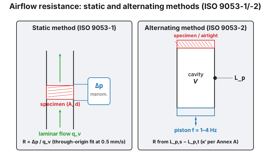
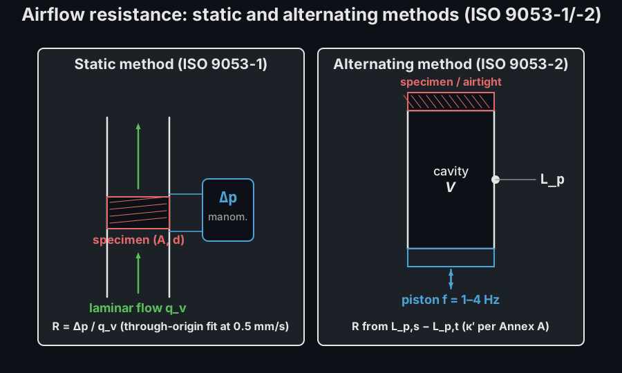
2. Static method (ISO 9053-1)

In the static method (ISO 9053-1:2018) a steady laminar flow is stepped up and the pressure difference plotted against the linear velocity $u=q_v/A$. A regression of at least second order constrained through the origin, $\Delta p=au+b{u}^2$, is fitted, and $\Delta p$ and $R_s$ are read at the reference velocity $u=0.5\text{mm/s}$ (Clause 7.5); the highest velocity must not exceed 15 mm/s. Because $R_s=\Delta p/u=a+bu$, the linear term $a$ is the zero-velocity specific airflow resistance.

Neither velocity is arbitrary, and Clause 7.5 says why. A plane wave of particle velocity 0.5 mm/s carries a sound pressure of 0.2 Pa — 80 dB — so the reference velocity puts the steady-flow rig at the amplitude the material will actually meet in use, which is the whole reason an aerodynamic measurement predicts an acoustic quantity. The 15 mm/s ceiling is the same arithmetic at 110 dB, and the standard warns that some materials are already non-linear there. That non-linearity is also why the fit is constrained through the origin and read at the bottom: $\Delta p$ must vanish with $u$, the linear coefficient $a$ is the viscous (Darcy) resistance acoustics wants, and the quadratic coefficient $b$ is the inertial correction that grows with velocity. One trap follows from the same clause: a textile “air permeability” to ISO 9237 is measured at velocities ten to a hundred times higher and therefore yields a different, larger resistivity, so a datasheet permeability figure can never be substituted for a measured $\sigma$ in the models of section 4.

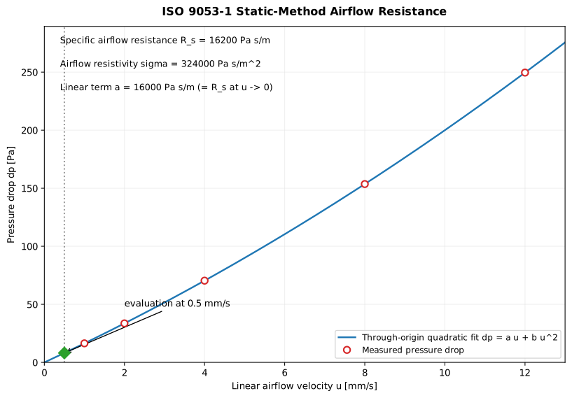
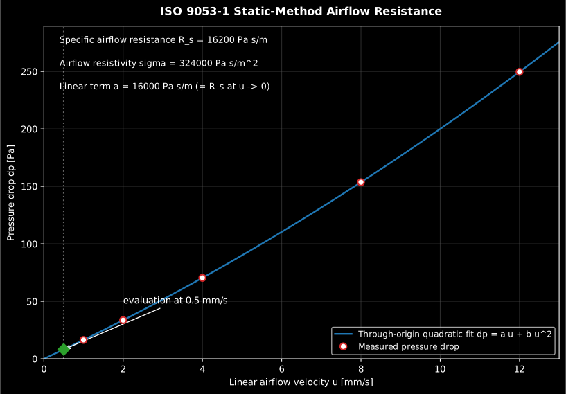
The slightly super-linear pressure drop is fitted through the origin; the specific airflow resistance is the fit read at 0.5 mm/s.

Show the code for this figure

import matplotlib.pyplot as plt
import numpy as np
from phonometry import materials

area = np.pi * 0.05**2                      # 100 mm diameter cell [m^2]
u = np.array([0.5, 1, 2, 4, 8, 12]) * 1e-3  # linear velocity [m/s]
dp = 1.6e4 * u + 4.0e5 * u**2               # measured pressure drop [Pa]
r = materials.static_airflow_resistance(u, dp, area=area, thickness=0.05)

u_fit = np.linspace(0.0, 13e-3, 200)
dp_fit = r.linear_coefficient * u_fit + r.quadratic_coefficient * u_fit**2
fig, ax = plt.subplots()
ax.plot(u_fit * 1e3, dp_fit, label="Through-origin fit  dp = a u + b u^2")
ax.plot(u * 1e3, dp, "o", label="Measured pressure drop")
ax.plot(r.evaluation_velocity * 1e3, r.pressure_drop, "D",
        label="Evaluation at 0.5 mm/s")
ax.set_xlabel("Linear airflow velocity u [mm/s]")
ax.set_ylabel("Pressure drop dp [Pa]")
ax.set_title(f"R_s = {r.specific_resistance:.0f} Pa·s/m")
ax.legend()
plt.show()

import numpy as np
from phonometry import materials

area = np.pi * 0.05**2            # 100 mm diameter cell [m^2]

# What the rig actually reads: a rotameter between the source and the specimen
# (in ml/min here) and a differential manometer. Clause 3.4 turns the first
# into the linear velocity the standard evaluates at.
q_v = np.array([236.0, 471.0, 942.0, 1885.0, 3770.0, 5655.0]) * 1e-6 / 60.0
u = np.array([materials.linear_airflow_velocity(q, area) for q in q_v])
print(np.round(u * 1e3, 2))       # [ 0.5  1.   2.   4.   8.  12. ] mm/s
dp = 1.6e4 * u + 4.0e5 * u**2                    # measured pressure drop [Pa]

r = materials.static_airflow_resistance(u, dp, area=area, thickness=0.05)
print(round(r.specific_resistance))   # 16200   R_s [Pa*s/m]
print(round(r.resistivity))           # 324000  sigma [Pa*s/m^2]
print(round(r.linear_coefficient))    # 16000   a = R_s at u -> 0
r.plot()   # the figure above: the fitted dp(u) with the evaluation point

# The same R_s straight from the pair the manometer and the rotameter give,
# without forming R first (Clause 3.2, second call form).
print(round(materials.specific_airflow_resistance(pressure_drop=8.1, velocity=0.5e-3)))

Those six flows are what a 100 mm cell needs to cover the clause’s range: the 0.5 mm/s reference velocity is 236 ml/min through that cross-section and the 15 mm/s ceiling is about 7 l/min, so the rotameter has to resolve a factor of thirty and land accurately at the bottom of it, where the evaluation happens. linear_airflow_velocity is scalar-only, hence the comprehension.

2.1 Running the static rig

The arithmetic above is the easy half. Everything that decides whether the number is right happens before the first flow step, and ISO 9053-1 spells it out in Clauses 5 to 7.

The specimen and the cell. The specimen must be wide enough to be representative: at least 10 pores across for a foam, 10 fibres for a fibrous material, 10 grains for a granular one, and where the microstructure is unknown, at least 95 mm in diameter or 90 mm on the smallest edge (Clause 6.2.1). The measurement cell has the same lateral dimensions as the specimen — its own floor is 29 mm (Clause 5.2) — and needs a free space of at least one diameter in front of the specimen so the flow arrives laminar and unidirectional, with more than a diameter behind it recommended for thin, low-porosity specimens. The specimen rests on a perforated support or a thin-wire grid with at least 50 % open area evenly distributed, holes no smaller than 3 mm, and an airflow resistance under 1 % of the specimen’s; Clause 5.2 even gives the closed form $R_s=8\eta h/(\varphi r^2)$ for a perforated plate so the support can be checked rather than assumed.

The two ways to get it wrong, and their signs. Both dominant error mechanisms are one-sided, which makes them diagnosable. A leak around the specimen rim is a resistance in parallel with the specimen, so the measured $R$ always comes out too low; Clause 7.2 seals the rim with a thin layer of petroleum jelly, thread seal tape or rings, and warns that the jelly must not penetrate the specimen, because inside the pores it does the opposite and reads high. Compression is the mirror image: $\sigma$ rises steeply with bulk density, so a specimen forced into the cell reads too high, repeatably and convincingly, which is why Clause 6.2.2 requires the thickness not to be modified when the specimen is placed in the cell. Thin specimens may be stacked only if the microstructure survives it, and for fibrous materials or non-wovens only with matching fibre orientation; where that is impossible, Annex A gives an impedance-tube route instead. The diagnostic worth remembering: a resistance that drifts downward as the flow rate rises is usually a leak opening under pressure, not material non-linearity, which pushes the other way.

In-position thickness. The thickness that defines $d$, and with it the tested bulk density, is measured with the specimen in the cell, by bringing the gauge into contact with the upper surface and compressing it lightly (Clauses 7.3 and 7.4) — not with a rule on the bench beforehand.

Instrument tolerances. The volumetric flow and the differential pressure must each be good to ±5 % of the indicated value (Clauses 5.4 and 5.5), the flow tap sits between the source and the specimen, and the pressure instrument must resolve down to 0.1 Pa — which the worked example above needs, since the whole reading at the reference velocity is 8.1 Pa. The flow source should reach 0.5 mm/s and hold it stable (Clause 5.3).

Is the rig itself usable? Clause 5.6 is the only check that answers that, and nothing in this library performs it: at least one calibrated test specimen shall be measured before a series of measurements, at least once a day, after any hardware or software change, and after any significant change of conditions — 0.5 kPa of pressure, 5 °C of temperature or 5 % of humidity. The artefact is normally made of straight cylindrical pores precisely because its resistance follows in closed form from the same $8\eta h/(\varphi r^2)$, so the check is against theory rather than against another laboratory, and the measured value must land within ±10 % of it. Record the check beside the measurement — the notes field of the fiche is the place — because the result object carries only the fit.

How much agreement to expect. Usually three specimens are measured (Clause 6.3), and Clause 8 puts the inter-laboratory reproducibility at around 15 % for open-cell foams, “strongly” worse for granular materials or materials with semi-closed pores, dominated by exactly the leakage and compression above. A 20 % disagreement with a catalogue value is therefore not evidence of a faulty instrument; a 20 % disagreement between your own three specimens is.

ISO 9053-1 report (.report())

StaticAirflowResult.report(path) renders a one-page PDF fiche laid out like an accredited airflow-resistance test report (ISO 9053-1:2018, static method): a standard-basis line, an optional metadata header block, a two-panel body with a metrics table (the evaluation velocity, the fitted pressure difference, the airflow resistance $R$, the specific airflow resistance $R_s$, the airflow resistivity $\sigma$ when a thickness is available, and the through-origin fit coefficients $a$ and $b$) beside the fitted $\Delta p(u)$ curve (the result’s own .plot()), the boxed specific airflow resistance $R_s$ with $R$ and $\sigma$ alongside, and a footer with the fixed disclaimer. ISO 9053-1 is a material characterisation, so the fiche carries no pass/fail verdict.

It uses the same ReportMetadata container and rendering engine as the other fiches. The descriptive fields that apply here are client, manufacturer, specimen, thickness (the specimen thickness $d$, in metres, shown in millimetres), test_room, test_date, temperature, relative_humidity, measurement_standard, laboratory, operator, report_id and notes. The requirement field is ignored (ISO 9053-1 has no verdict). The fiche embeds the fitted curve, so rendering needs both reportlab and matplotlib (pip install "phonometry[report,plot]"); only engine="reportlab" is supported. The fiche renders in English by default; pass language="es" for a Spanish fiche (translated fixed strings and a comma decimal separator).

from phonometry import materials, ReportMetadata

r = materials.static_airflow_resistance(u, dp, area=area, thickness=0.05)
r.report(
    "airflow_fiche.pdf",
    metadata=ReportMetadata(
        specimen="50 mm porous absorber (open-cell)",
        thickness=0.050,
        measurement_standard="ISO 9053-1",
        test_room="Static airflow rig, 100 mm cell",
        laboratory="Phonometry Reference Laboratory",
    ),
)                                  # R_s, R and sigma at u = 0.5 mm/s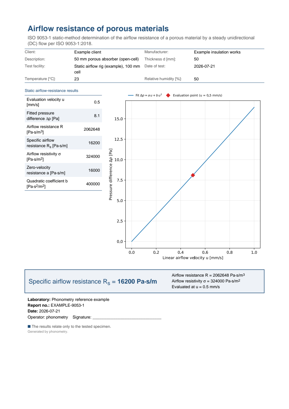

One-page static airflow-resistance fiche: a metadata header (client, manufacturer, specimen, specimen thickness, test facility, temperature and humidity), a metrics table with the evaluation velocity, the fitted pressure difference, the airflow resistance R, the specific airflow resistance R_s, the airflow resistivity sigma and the through-origin fit coefficients a and b beside the fitted pressure-drop curve, and the boxed specific airflow resistance R_s with R and sigma alongside, read at the 0.5 mm/s reference velocity.

Download the report (PDF)

Static airflow-resistance fiche (StaticAirflowResult.report), R_s, R and sigma at 0.5 mm/s.

3. Alternating method (ISO 9053-2)

In the alternating method (ISO 9053-2:2020) a piston oscillating at 1–4 Hz drives an alternating flow into a cavity terminated either by the specimen or by an airtight plug; the resistance follows from the sound-pressure-level difference between the two terminations (Formula (2)):

$$R=\frac{{\kappa }^{\prime }{P}_S}{2\pi fV}\cdot \frac{h_t}{h_s}\cdot 10^{(L_{p,s}-L_{p,t})/20},$$

with $P_S$ the static (atmospheric) pressure, $f$ the piston frequency, $V$ the volume of the air cavity (including every connecting pipe, with the piston at mid-stroke), $L_{p,s}$ and $L_{p,t}$ the cavity sound pressure levels measured with the measurement cell carrying the specimen and with the airtight termination, $h_s$ and $h_t$ the corresponding piston stroke amplitudes, and ${\kappa }^{\prime }$ the effective ratio of specific heats.

What the formula is saying. The airtight termination is the reference: with it the cavity is a sealed compliance, the piston’s whole swept volume goes into compressing the air, and the level is high. Put the specimen in its place and most of that flow bleeds through the pores instead, so the cavity level falls — and the drop $L_{p,t}-L_{p,s}$ is the measurement. The stroke ratio $h_t/h_s$ only normalises the two runs to the same volume velocity, which is why the two strokes are deliberately unequal: ISO 9053-2 Clause 6.2 NOTE 1 gives 1.4 mm with the airtight termination against 14 mm with the specimen for a 10 mm piston, a 100 mm cell and a cavity near $10^{-3}$ m³ — exactly the example below — so that both levels land inside the analyser’s useful range. Two consequences are worth having. Only a level difference at one frequency enters, so the sound measuring device needs no absolute calibration and its frequency response is not critical; what matters is level linearity (Clause 8.7). And the run order is fixed by Clause 8.5/8.6: measure $P_S$, set the stroke to $h_s$, read the piston frequency, the background level $L_{p,b}$ (source running, neither cell nor termination fitted) and then $L_{p,s}$; only then swap in the airtight termination, set $h_t$, confirm the frequency has not moved, and read $L_{p,t}$.

Heat conduction between the oscillating air and the cavity walls makes the compression not fully adiabatic; the normative Annex A corrects $\kappa$ down to

$${\kappa }^{\prime }=\frac{\kappa }{\sqrt{1+(\kappa -1)\frac{S}{V}b+\frac{1}{2}((\kappa -1)\frac{S}{V}b{)}^2}},b=\sqrt{\frac{2c_0{l}_h}{\omega }},l_h=\frac{k_a}{{\rho }_0{c}_0{C}_P},$$

with $S$ and $V$ the cavity surface and volume, $b$ the thermal boundary-layer thickness (thermal_boundary_layer_thickness), $l_h$ the characteristic thermal diffusion length built from the thermal conductivity $k_a$, the density ${\rho }_0$, the speed of sound $c_0$ and the specific heat at constant pressure $C_P$, and $\omega =2\pi f$. For the Annex A.3 example cavity this gives ${\kappa }^{\prime }=1.370$, about 2 % below the adiabatic 1.4008.

from phonometry import materials

# Annex A.3 cavity: closed cylinder 100 mm x 100 mm, piston at 2 Hz
kp = materials.effective_kappa(cavity_surface=0.0471, cavity_volume=7.854e-4, frequency=2.0)
print(round(kp, 3))               # 1.37   effective ratio of specific heats
print(round(materials.thermal_boundary_layer_thickness(2.0) * 1e3, 2))   # 1.83 mm

R = materials.alternating_airflow_resistance(
    level_specimen=74.0, level_termination=90.0,
    piston_stroke_specimen=14e-3, piston_stroke_termination=1.4e-3,
    frequency=2.0, cavity_volume=7.854e-4, kappa_prime=kp,
)
print(round(R))                   # 222956  airflow resistance R [Pa*s/m^3]

$b$ is 1.83 mm at 2 Hz — millimetre-scale, against a cavity 100 mm across. That is why ${\kappa }^{\prime }$ enters through the surface-to-volume ratio $S/V$ and not through the cavity’s absolute size: only the air within a boundary layer of the wall exchanges heat with it, so a rig scaled down at constant shape keeps the same $b$ while $S/V$ grows, and the correction grows with it.

Pass the effective_kappa result to alternating_airflow_resistance for an Annex-A-conforming figure; its kappa_prime argument otherwise defaults to the uncorrected adiabatic 1.4.

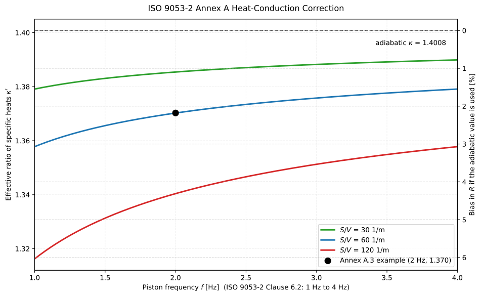
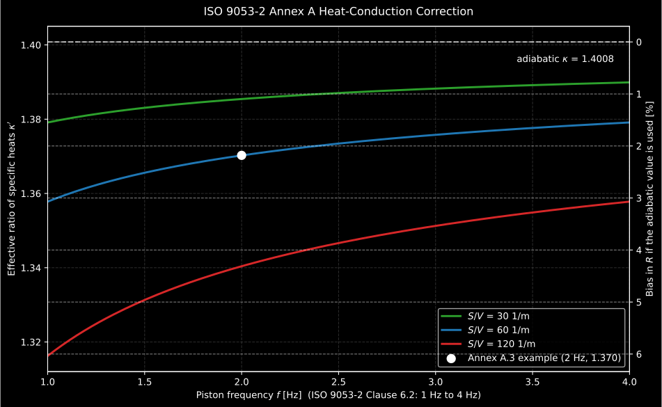
The Annex A correction over the whole 1–4 Hz piston band. It falls as the frequency falls (a thicker boundary layer reaches more of the air) and rises with the cavity’s surface-to-volume ratio, which is the only geometric quantity it depends on. For the Annex A.3 cavity — $S/V=60$ 1/m — the correction is about 2 %, and since $R$ is proportional to ${\kappa }^{\prime }$, skipping it biases every reported resistance by that much. A cavity twice as compact doubles the penalty, so a scaled-down rig cannot treat the correction as optional.

Show the code for this figure

import matplotlib.pyplot as plt
import numpy as np

f = np.linspace(1.0, 4.0, 120)
for s_over_v in (30.0, 60.0, 120.0):
    volume = 7.854e-4                      # the Annex A.3 cavity volume
    kappa = [materials.effective_kappa(cavity_surface=s_over_v * volume,
                                       cavity_volume=volume, frequency=fi)
             for fi in f]
    plt.plot(f, kappa, label=f"S/V = {s_over_v:g} 1/m")
plt.axhline(1.4008, ls="--", label="adiabatic 1.4008")
plt.plot([2.0], [materials.effective_kappa(cavity_surface=0.0471,
                                           cavity_volume=7.854e-4,
                                           frequency=2.0)], "D")
plt.xlabel("Piston frequency f [Hz]")
plt.ylabel("Effective ratio of specific heats")
plt.legend()
plt.show()

Acceptance criteria (Clause 8.7). Formula (2) is only valid when two conditions hold. Formula (3), $(h_t/h_s)10^{(L_{p,s}-L_{p,t})/20}<0.3$, keeps the linearised Formula (2) close enough to the exact relation of Annex B; Formula (4), $L_{p,s}-L_{p,b}>10$ dB, keeps the background’s influence on $L_{p,s}$ below 0.4 dB for uncorrelated noise (a correlated background needs more). alternating_airflow_resistance accepts background_level precisely so it can check the second, and warns through AirflowResistanceWarning when either fails or when the piston frequency leaves 1–4 Hz. When one does fail, the standard offers four knobs: change the specimen length, the specimen diameter, the cavity volume, the piston frequency or the piston stroke. It is also worth checking that the flow the piston drives through the specimen lands in the recommended window: Clause 6.2 gives $q_v=2\pi fh{A}_P$ and Formula (1) $v_s=q_v/A$, and recommends rms velocities between 0.5 mm/s and 4 mm/s — the same physical regime as the static method’s reference velocity.

# The same run, with the background level so the Formula (4) check is live,
# and the flow the piston actually drives through a 100 mm cell.
R = materials.alternating_airflow_resistance(
    level_specimen=74.0, level_termination=90.0,
    piston_stroke_specimen=14e-3, piston_stroke_termination=1.4e-3,
    frequency=2.0, cavity_volume=7.854e-4, kappa_prime=kp,
    background_level=52.0,          # Formula (4): 74.0 - 52.0 = 22 dB > 10 dB
)
piston_area = np.pi * 0.005**2                          # 10 mm piston
q_s = materials.piston_volume_flow_rate(2.0, 14e-3, piston_area)
print(round(q_s / area * 1e3, 2))   # 1.76 mm/s, inside the 0.5-4 mm/s window

# Formula (3): the ratio the standard caps at 0.3.
print(round((1.4e-3 / 14e-3) * 10 ** ((74.0 - 90.0) / 20), 3))   # 0.016

# Finish the chain the static method gets for free: R -> R_s -> sigma.
r_s = materials.specific_airflow_resistance(R, area)
print(round(r_s, 1), round(r_s / 0.05))    # 1751.1 Pa*s/m, 35022 Pa*s/m^2

What Part 2 returns, and what it does not. Unlike the static method, alternating_airflow_resistance returns a bare resistance in Pa·s/m³, not a result object: there is no StaticAirflowResult equivalent, so no .plot() and no ISO 9053-2 fiche, and the two steps to $R_s$ and $\sigma$ are the caller’s — which is what the last two lines above do. What Part 2 buys instead is the specimens Part 1 cannot hold: very open or very thin materials whose static pressure drop is too small to read against the rig’s own leakage, and delicate or granular samples a steady flow would deform or displace. The two methods should agree inside the reproducibility quoted above when the specimen is properly sealed, with one documented exception — ISO 9053-2 Clause 5 NOTE warns that for materials whose visco-inertial transition frequency lies below 100 Hz (coarse metal or plant fibres, low-porosity foams with big pores, coarse road pavements) the static method can legitimately give a different answer. Part 1 remains the reference method whenever a stable static reading is possible.

4. What the resistivity feeds

The flow resistivity is not an end in itself: almost every consumer of the number is a porous-material model. The empirical Delany-Bazley and Miki regressions predict a porous material’s complex characteristic impedance and wavenumber from $\sigma$ alone, through the dimensionless ratio $X={\rho }_{0}f/\sigma$; the physics-based Johnson-Champoux-Allard model keeps $\sigma$ as the first of its five parameters. Fitted to a tube or reverberation-room measurement once, those models then predict the layer at any thickness, backing or incidence angle. The whole model family, and the multilayer solver that stacks the layers, lives in Porous and Multilayer Absorbers; the regression validity window of Delany-Bazley ($0.01<X<1$) is stated there in the same $X$ that $\sigma$ defines.

Because $\sigma$ enters the models as a ratio, its useful range is bounded on both sides. A layer with too little resistivity barely couples to the sound field: air moves through it freely and little energy is dissipated. Too much resistivity and the layer behaves like a wall: the wave reflects off the front face before the pores can absorb it. Between the two lies the classic design window for the total flow resistance of a layer of thickness $d$,

$${\rho }_0{c}_0\lesssim R_s=\sigma d\lesssim 4{\rho }_0{c}_0,$$

that is, a specific flow resistance of one to four times the characteristic impedance of air (${\rho }_0{c}_0\approx 410$ Pa·s/m). A 50 mm blanket therefore wants a resistivity of roughly 8 kPa·s/m² to 33 kPa·s/m², which is exactly where commercial absorber products cluster.

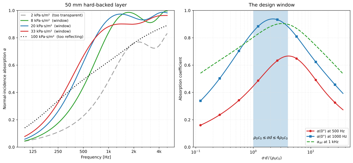
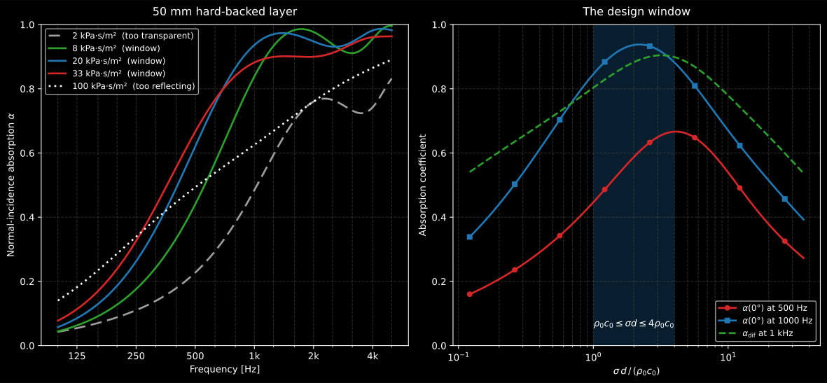
The window, drawn. Left: the same 50 mm hard-backed layer at five resistivities. The 2 kPa·s/m² layer is too transparent everywhere — the wave passes through it, reflects off the wall and comes back out. The 100 kPa·s/m² one leads below about 400 Hz, where more resistance still helps, and then saturates near 0.89 while the three window curves reach 1: above 1 kHz the wave is reflecting off the face before the pores can act. Right: the same family read against the dimensionless $\sigma d/({\rho }_0{c}_0)$, with the $1$ to $4$ window shaded. The optimum is flat-topped, which is the practical point — a catalogue spread of tens of percent inside the window costs almost nothing, and the same spread just outside it costs a great deal. Note also that the diffuse-field curve peaks lower on the axis than the normal-incidence one, so a layer optimised in the tube is slightly over-resistive for a room. The window is engineering guidance and forms no part of either ISO 9053 part.

Show the code for this figure

f_win = np.geomspace(100.0, 5000.0, 200)
for sigma in (2e3, 8e3, 20e3, 33e3, 100e3):
    layer = materials.layered_absorber(
        f_win, [materials.PorousLayer(0.05, materials.miki(f_win, sigma))]
    )
    plt.semilogx(f_win, layer.absorption, label=f"{sigma/1e3:g} kPa s/m^2")
plt.xlabel("Frequency [Hz]")
plt.ylabel("Normal-incidence absorption")
plt.legend()
plt.show()

The worked specimen of section 2 is a useful counter-example: its 324 kPa·s/m² is an order of magnitude above the top of the window, so at 50 mm it is not a bulk absorber at all but a resistive facing, of the kind that belongs in front of a cavity rather than alone against a wall.

Typical orders of magnitude, for orientation rather than design: glass wools run from a few kPa·s/m² in light thermal grades to some tens of kPa·s/m² in dense acoustic boards; rock wools sit somewhat higher at equal density; open-cell foams (melamine, polyurethane) span roughly 5 kPa·s/m² to 30 kPa·s/m²; and fibrous felts and compressed boards can exceed 100 kPa·s/m², at which point they act more as resistive facings than as bulk absorbers. Within one product family the resistivity rises steeply with bulk density and falls with fibre diameter, which is why nominally identical products from two production runs can differ by tens of percent, and why a measured $\sigma$, not a catalogue value, should anchor any model fit that will be trusted quantitatively.

The number also travels beyond the porous models. The perforated-panel and microperforated-panel impedances contain the same viscous physics evaluated in a single hole; the slit absorber inherits it per slit; and when an impedance tube measurement disagrees with a model prediction, the first parameter to re-measure, before touching the model, is $\sigma$.

What this guide covers

• Covered

  Both parts of ISO 9053: the static method of Clause 7.5 (static_airflow_resistance, the through-origin regression and the 0.5 mm/s evaluation velocity) and the alternating method of ISO 9053-2 Formula (2) with the Annex A effective ratio of specific heats (effective_kappa, thermal_boundary_layer_thickness, alternating_airflow_resistance), including the 1-4 Hz and Formula (3)/(4) validity warnings, and the accredited-style ISO 9053-1 fiche. The definitional conversions that connect them to what a rig reads are linear_airflow_velocity (Clause 3.4), specific_airflow_resistance (Clause 3.2, in both call forms) and piston_volume_flow_rate (ISO 9053-2 Clause 6.2).

• Not covered

  The equivalent-fluid models that consume the resistivity (Delany-Bazley, Miki, Johnson-Champoux-Allard) live in Porous and Multilayer Absorbers, and the $\sigma d$ design window of section 4 is engineering guidance, not part of either standard. ISO 9053-1 defines no pass/fail verdict or single-number rating, so the fiche carries neither.

See also

• Porous and Multilayer Absorbers: the Delany-Bazley, Miki and Johnson-Champoux-Allard models that consume the resistivity, and the multilayer transfer-matrix solver.
• Impedance Tube: the normal-incidence measurement that a $\sigma$-anchored model is usually fitted against.
• Sound Absorption Measurement and Rating: the reverberation-room measurement and the ISO 11654 rating of the finished absorber.
• API reference: materials.absorbers.airflow_resistance.
• Theory: Acoustic material characterisation: the ISO 9053 definitions of resistance, resistivity and the flow regime they assume.

References

• Allard, J. F., & Atalla, N. (2009). Propagation of sound in porous media: Modelling sound absorbing materials (2nd ed.). Wiley. https://doi.org/10.1002/9780470747339The porous-material theory that consumes the measured resistivity: viscous and thermal dissipation in the pores, and the equivalent-fluid models of section 4. ISBN 978-0-470-74661-5.
• International Organization for Standardization. (2018). Acoustics — Determination of airflow resistance — Part 1: Static airflow method (ISO 9053-1:2018). The static method of section 2, with the through-origin regression and the 0.5 mm/s reference velocity.
• International Organization for Standardization. (2020). Acoustics — Determination of airflow resistance — Part 2: Alternating airflow method (ISO 9053-2:2020). The alternating method of section 3, with the Annex A effective ratio of specific heats, validated against the standard's own Annex A.3 worked example.