Porous and Multilayer Absorbers

Given a porous material’s flow resistivity (the quantity the flow rig measures) the classical equivalent-fluid models predict its complex characteristic impedance and wavenumber, and a transfer-matrix stack of layers (porous blankets, air gaps, perforated and microperforated panels, membranes) predicts the absorption coefficient of the whole construction before anything is built. This page covers the three porous models (Delany–Bazley, Miki, Johnson–Champoux–Allard), the multilayer solver, the resonant sheet layers of Maa and the random-incidence (Paris) integral. All three of those models assume the skeleton never moves; the page also covers what to do when it does — the limp-frame inertia correction below the decoupling frequency, and the full Biot poroelastic layer, whose frame-borne wave produces a quarter-wavelength resonance no equivalent fluid can reproduce. The measurement counterparts live in the impedance tube and reverberation room guides; rating the predicted spectrum lives in the latter’s ISO 11654 section; and the resonant metamaterial relatives of these constructions, slow-sound slit panels that reach perfect absorption at critical coupling, have their own guide, Metamaterial Absorbers.

1. Equivalent-fluid models of a porous material

A rigid-frame porous material behaves like an equivalent fluid with a complex characteristic impedance $Z_c$ and wavenumber $k$ (time convention $e^{+j\omega t}$, so a passive medium has $\mathrm{Im}(k)<0$).

Delany–Bazley (Mechel 2e Sect. G.11; Bies 5e Appendix D, Table D.1; Hopkins Eqs. 1.171–1.174) is the one-parameter power law in the absorber variable $X={\rho }_{0}f/\sigma$:

$$\frac{Z_c}{{\rho }_0{c}_0}=1+C_1{X}^{-C_2}-j{C}_3{X}^{-C_4},\frac{k}{k_0}=1+C_5{X}^{-C_6}-j{C}_7{X}^{-C_8},$$

with the classic rockwool/fibreglass coefficients $(0.0571,0.754,0.087,0.732,0.0978,0.700,0.189,0.595)$ and a stated fit range $0.01<X<1.0$ (porosity close to one). The library also ships the Table D.1 presets fitted to polyester ("garai_pompoli") and to foams ("dunn_davern", "wu"). Outside the fit range a PorousAbsorberWarning is raised and the extrapolated values are still returned; the classic failure is a negative real part of the layer input impedance at low frequency (Mechel Sect. G.12).

Miki (1990) refitted the same Delany–Bazley data under a passivity (positive-real) constraint, so the model stays physically well behaved below the fit range; it is the usual choice when a one-parameter model must be evaluated broadband. Miki states his own validity window in the paper’s variable $Y=f/\sigma$, $0.01<Y<1.0$ — the Delany–Bazley window divided by ${\rho }_0$, so the two differ by a factor of about 1.2 rather than by a slip of the pen. The library warns on $X$ for delany_bazley and on $Y$ for miki, each against its own published range.

Johnson–Champoux–Allard (JCA) is the five-parameter semi-phenomenological model (Cox & D’Antonio 3e Eqs. 6.19–6.25): flow resistivity $\sigma$, porosity $\varphi$, tortuosity ${\alpha }_{\infty }$ and the viscous/thermal characteristic lengths $\Lambda$, ${\Lambda }^{\prime }$ give the effective density and bulk modulus with the exact limits $j\omega {\rho }_e\to \sigma$ at DC, ${\rho }_e\to ({\alpha }_{\infty }{\rho }_0/\varphi )(1+(1-j){\delta }_v/\Lambda )$ at high frequency, and the isothermal-to-adiabatic transition in $K_e$.

import numpy as np
from phonometry import materials

f = np.geomspace(200.0, 4000.0, 200)
db = materials.delany_bazley(f, 20000.0)          # sigma in Pa s/m2
mk = materials.miki(f, 20000.0)
jca = materials.johnson_champoux_allard(
    f, 20000.0, porosity=0.98, tortuosity=1.0,
    viscous_length=8.7e-5, thermal_length=8.7e-5,
)
print(np.round(db.normalized_impedance[0], 3))    # (2.598-2.209j)
print(np.round(mk.normalized_impedance[0], 3))    # (2.286-1.965j)
print(np.round(jca.normalized_impedance[0], 3))   # (2.321-2.075j)

db.plot()   # normalised Zc and k components vs frequency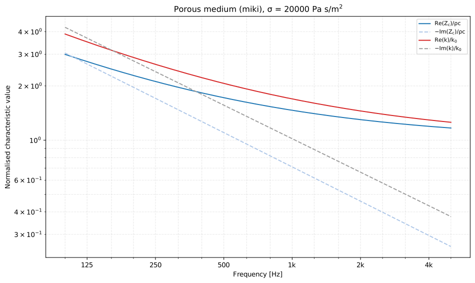

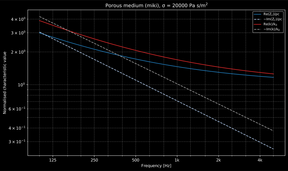
The classical presentation of an equivalent-fluid model (Cox & D’Antonio 3e, Figs. 6.19–6.20): at low frequency the viscous forces dominate and the material looks stiff and lossy (all four components large); as frequency rises the components fall towards the free-air limits $Z_c\to {\rho }_0{c}_0$ and $k\to k_0$, so a thin layer only works where its thickness is a fair fraction of the wavelength inside the material.

Show the code for this figure

import matplotlib.pyplot as plt
import numpy as np
from phonometry import materials

f = np.geomspace(100.0, 5000.0, 260)
mk = materials.miki(f, 20000.0)          # sigma = 20 kPa s/m^2

# One line: normalised Zc and k components on a log-log grid.
mk.plot()
plt.show()

# By hand, from the result's fields:
fig, ax = plt.subplots()
ax.loglog(f, mk.normalized_impedance.real, label="Re(Zc)/rho c")
ax.loglog(f, -mk.normalized_impedance.imag, "--", label="-Im(Zc)/rho c")
ax.loglog(f, mk.normalized_wavenumber.real, label="Re(k)/k0")
ax.loglog(f, -mk.normalized_wavenumber.imag, "--", label="-Im(k)/k0")
ax.set(xlabel="Frequency [Hz]", ylabel="Normalised characteristic value")
ax.legend()
plt.show()

The three models agree closely over the Delany–Bazley fit range (Cox & D’Antonio Figs. 6.19–6.21 make the same comparison); JCA extends the prediction physically outside it. A PorousMediumResult built from measured data (for example the $Z_c$, $k$ recovered by the ASTM E2611 transfer-matrix reduction) plugs into the layer solver exactly like a modelled one.

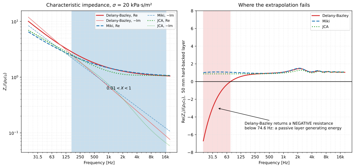
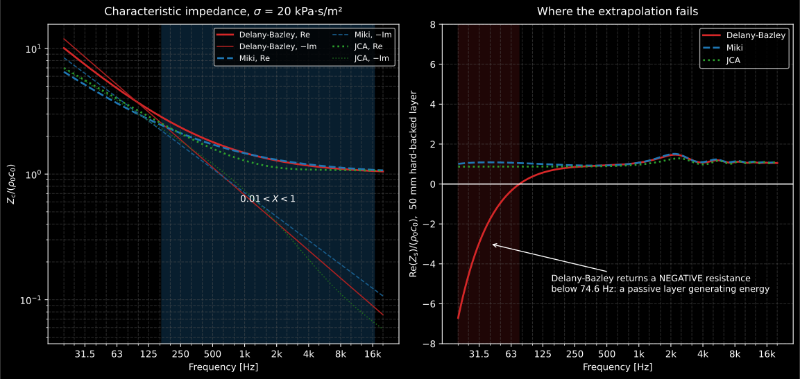
The three models, and what “outside the fit range” costs. Inside the $0.01<X<1$ window the curves are practically the same material — which is why the one-parameter fits are still used. Below it they part company, and the right panel shows the consequence in the quantity a designer actually uses: for this 50 mm hard-backed layer Delany–Bazley returns a negative resistance below 74.6 Hz, a passive layer that generates energy. Miki’s passivity constraint keeps it positive, and JCA is physical everywhere by construction. The warning PorousAbsorberWarning fires here; the extrapolated values are still returned, so it is the caller’s job to notice.

Show the code for this figure

f_cmp = np.geomspace(20.0, 20000.0, 400)
for name, medium in (
    ("Delany-Bazley", materials.delany_bazley(f_cmp, 20000.0)),
    ("Miki", materials.miki(f_cmp, 20000.0)),
):
    zs = materials.layered_absorber(
        f_cmp, [materials.PorousLayer(0.05, medium)]
    ).normalized_impedance
    below = f_cmp[zs.real < 0.0]
    print(name, "Re(Zs) < 0 below", f"{below.max():.1f} Hz" if below.size else "never")
# Delany-Bazley Re(Zs) < 0 below 74.6 Hz
# Miki Re(Zs) < 0 never

1.1 Where the five JCA numbers come from

Delany–Bazley and Miki need one measured number. JCA needs five, and a reader with a real sample has to get the other four from somewhere.

Flow resistivity $\sigma$ is the only one with a standard behind it: ISO 9053-1 or -2, in the airflow-resistance guide. It is also the one to re-measure first when a model and a measurement disagree.

Porosity $\varphi$ is the open (connected) porosity — the ratio of the air volume to the total volume, counting only air that is not locked inside the frame, so a closed bubble in a foam belongs to the frame and not to $\varphi$ (Allard & Atalla 2e Sect. 2.5.1). It is measured by gas-displacement methods (Zwikker & Kosten 1949; Champoux et al. 1991), and for most fibrous materials and open-cell foams it “lies very close to 1”, which is why 0.95–0.99 is a defensible starting guess and why $\varphi$ is rarely the parameter that matters.

Tortuosity ${\alpha }_{\infty }$ is an intrinsic property of the micro-geometry: it is what the effective density tends to, times ${\rho }_0$, once the viscous skin depth vanishes. It can be evaluated from electrical-conductivity measurements on a frame saturated with a conducting fluid (Sect. 4.9), or together with the two characteristic lengths from ultrasonic transmission (Sect. 5.3.5). It is 1 for straight pores normal to the surface and grows with any dispersion of the microscopic velocity.

The characteristic lengths $\Lambda$, ${\Lambda }^{\prime }$ are the hardest to get directly: the reference method is ultrasonic transmission in two gases (helium and air), and the book’s own worked foam — $\varphi =0.98$ — comes out at $\Lambda =202$ µm, ${\Lambda }^{\prime }=367$ µm and ${\alpha }_{\infty }=1.05$ from exactly that measurement (Leclaire et al. 1996, reproduced as Fig. 5.5). Note the ratio: ${\Lambda }^{\prime }/\Lambda \approx 1.8$ there, not 1 and not 3. It is a property of the pore geometry, so treat it as something to find, not to assume. Where no ultrasonic bench is available, the practical route is an inverse fit against a measured normal-incidence surface impedance — the quantity the impedance tube returns — and where even that is out of reach, the closed-form fallback $\Lambda ={\Lambda }^{\prime }=\sqrt{8{\alpha }_{\infty }\eta /(\varphi \sigma )}$ with ${\alpha }_{\infty }=1$ collapses JCA back onto Delany–Bazley over its fit range.

The inverse fit is a few lines, and it is worth running against a synthetic “measurement” first so that the recovery can be checked:

from scipy.optimize import least_squares

f_fit = np.geomspace(200.0, 1600.0, 40)      # a 100 mm tube's usable band

def surface_impedance(sigma, viscous):
    """Normalised Zs of a 50 mm hard-backed JCA layer."""
    medium = materials.johnson_champoux_allard(
        f_fit, sigma, porosity=0.98, tortuosity=1.05,
        viscous_length=viscous, thermal_length=2.5 * viscous,
    )
    layer = materials.layered_absorber(f_fit, [materials.PorousLayer(0.05, medium)])
    return layer.normalized_impedance

# Stand in for the tube result: a specimen whose true parameters we know.
measured = surface_impedance(22000.0, 9.0e-5)

def residual(p):                              # sigma in kPa s/m2, Lambda in um
    z = surface_impedance(p[0] * 1e3, p[1] * 1e-6)
    return np.concatenate([(z - measured).real, (z - measured).imag])

fit = least_squares(residual, x0=[10.0, 50.0],
                    bounds=([1.0, 10.0], [200.0, 500.0]))
print(round(fit.x[0] * 1e3), round(fit.x[1], 1))   # 22000 90.0 -- both recovered

Two warnings go with it. Fitting all five parameters at once is under-determined against one impedance spectrum: hold $\varphi$ at its measured or near-unity value, hold ${\alpha }_{\infty }$ unless there is a reason to move it, and let the fit find $\sigma$ and the lengths. And when a fitted $\sigma$ comes out far from the flow rig’s answer, believe the rig: a fit that has absorbed a mounting error into the material parameters will predict every other construction wrong.

Limp frames: when the skeleton moves (Allard & Atalla 11.3.4)

Every model above assumes the frame stands still. That is only true above the decoupling frequency of Zwikker and Kosten,

$$F_d=\frac{\sigma {\varphi }^2}{2\pi {\rho }_1},$$

with ${\rho }_1$ the bulk density of the frame (the density of the sample as weighed, not of the material the fibres are made of). Below $F_d$ the visco-inertial coupling is strong enough for the wave in the pores to drag the frame along, and a light frame (aeronautic-grade fibreglass, felts, thin screens) has real inertia to contribute. Neglecting the stiffness of the frame but not its mass in the Biot mixed pressure-displacement formulation leaves an equivalent fluid with the same bulk modulus and a corrected effective density (Allard & Atalla 2e Eqs. 11.53-11.55, after Panneton 2007):

$${\tilde{\rho }}_{\text{limp}}=\frac{{\rho }_t{\tilde{\rho }}_{\text{eq}}-{\rho }_0^2}{{\rho }_t+{\tilde{\rho }}_{\text{eq}}-2{\rho }_0},{\rho }_t={\rho }_1+\varphi {\rho }_0,$$

where ${\tilde{\rho }}_{\text{eq}}$ is the rigid-frame effective density of any of the three models above and ${\rho }_t$ is the apparent total density of the material. What that form is anchored on, and how weakly, is set out in the validation note at the end of this subsection. It has two limits worth knowing as physics:

• heavy frame: as ${\rho }_1$ grows the correction vanishes and the rigid-frame result comes back;
• low frequency: the rigid-frame density diverges as $\sigma /(j\omega )$, while the limp one converges on the finite, real ${\rho }_t$. A rigid frame forbids rigid-body motion of the sample; a limp one allows it, which is why the limp model is the right one for an unconstrained specimen in an impedance tube.

limp_frame takes a PorousMediumResult and returns another one, so it drops straight into a PorousLayer in the stack.

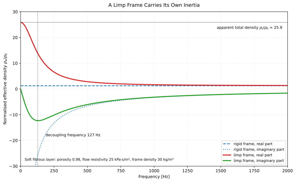
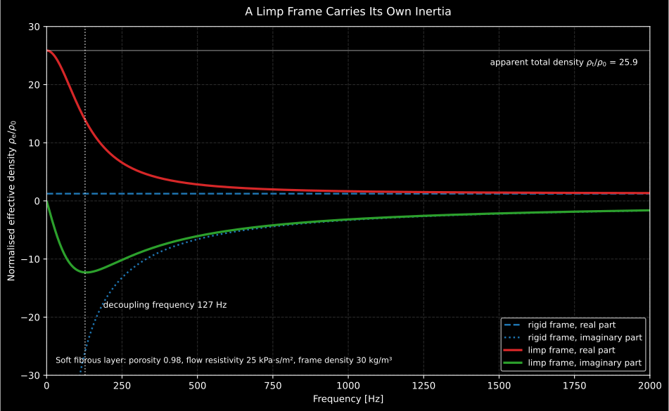
The same 50 mm soft fibrous layer under both models (Allard & Atalla Table 11.2, the input set behind their Fig. 11.2). Above the decoupling frequency the two predictions are indistinguishable, which is the plot’s own check on the correction; below it the rigid-frame effective density runs away and the limp one settles on ${\rho }_t/{\rho }_0=25.9$.

Show the code for this figure

import matplotlib.pyplot as plt
import numpy as np
from phonometry import (
    PorousLayer, decoupling_frequency, johnson_champoux_allard,
    layered_absorber, limp_frame, limp_frame_applicable,
)

# Allard & Atalla Table 11.2: soft fibrous layer, 50 mm.
f = np.linspace(1.0, 2000.0, 800)
rigid = johnson_champoux_allard(
    f, 25e3, porosity=0.98, tortuosity=1.02,
    viscous_length=90e-6, thermal_length=180e-6,
)
limp = limp_frame(rigid, frame_density=30.0, porosity=0.98)

print(round(decoupling_frequency(25e3, porosity=0.98, frame_density=30.0), 1))
# 127.4
print(round(float(limp.effective_density[0].real), 1))     # 31.2 = rho_t
print(limp_frame_applicable(20e3), limp_frame_applicable(25e3))  # True False

limp.plot()   # normalised Zc and k of the corrected medium
plt.show()

# By hand, the Fig. 11.2 view:
rho0 = rigid.air_density
fig, ax = plt.subplots()
for medium, style in ((rigid, "--"), (limp, "-")):
    ax.plot(f, medium.effective_density.real / rho0, style)
    ax.plot(f, medium.effective_density.imag / rho0, style)
ax.set(xlabel="Frequency [Hz]", ylabel="rho_e / rho_0", ylim=(-30, 30))
plt.show()

The correction is only worth applying where the frame really is limp. Beranek (1947) asked for $|K_c/K_f|<0.05$ between the bulk modulus of the frame in vacuum and that of the fluid in the pores; the frame-structural-interaction study of Doutres et al. (2007) relaxed that to $0.2$, which for air ($K_f\approx P_0=101.3$ kPa) is the rule of thumb that the frame must be softer than about 20 kPa. limp_frame_applicable applies either threshold. Neither accounts for mounting: a thin light foam decoupled from a vibrating structure by an air gap behaves limply well above the limit, and a material bonded to a vibrating structure should not be treated as rigid-framed at all.

The practical consequence, for the 50 mm layer above with a rigid backing, is a lower absorption coefficient in the bottom two thirds of an octave and a slightly higher one either side of 500 Hz:

import numpy as np
from phonometry import (
    PorousLayer, johnson_champoux_allard, layered_absorber, limp_frame,
)

bands = np.array([100, 125, 160, 200, 250, 315, 400, 500, 1000], dtype=float)
rigid = johnson_champoux_allard(
    bands, 25e3, porosity=0.98, tortuosity=1.02,
    viscous_length=90e-6, thermal_length=180e-6,
)
limp = limp_frame(rigid, frame_density=30.0, porosity=0.98)
for medium in (rigid, limp):
    print(layered_absorber(bands, [PorousLayer(0.05, medium)]).absorption.round(2))
# [0.07 0.11 0.17 0.24 0.32 0.43 0.54 0.64 0.88]   rigid frame
# [0.04 0.08 0.15 0.24 0.36 0.48 0.61 0.71 0.91]   limp frame

Honest note on validation. Allard & Atalla contains exactly one table of computed numbers in the whole book, and it is not a surface impedance: every prediction-versus-measurement pair in the porous chapters, Fig. 11.2 included, is a figure. No published source checked (Allard & Atalla itself, Cox & D’Antonio, Mechel, and the round-robin and Biot literature) tabulates the quantity either. The anchor is therefore the printed Eq. 11.55 itself, transcribed term by term against the printed page. The two exact limits the book states in prose (heavy frame and $\omega \to 0$) are checked as well, but they are weaker than they look: a sign-flipped variant of the equation satisfies both, and reproduces the $1/{\rho }_1$ decay of the heavy-frame residual too, so the limits cannot tell the printed form from that variant. The decoupling frequency evaluated on the fully specified glass wool of their Table 6.1, where pure arithmetic gives 43.27 Hz, is independent of all this.

Elastic frames: the full Biot layer (Allard & Atalla 6 and 11)

The limp model throws the frame stiffness away. Keep it, and the porous layer stops being a fluid: the Biot theory treats the skeleton as an elastic solid coupled to the pore fluid through a potential coupling coefficient $Q$ and an inertial coupling coefficient, and predicts three waves in an isotropic material instead of one. Two are compressional and one is shear (Allard & Atalla 2e ch. 6). The stress-strain relations are

$${\sigma }_{ij}^s=\left[(P-2N){\theta }^s+Q{\theta }^f\right]{\delta }_{ij}+2N{e}_{ij}^s,{\sigma }_{ij}^f=-\varphi p{\delta }_{ij}=(Q{\theta }^s+R{\theta }^f){\delta }_{ij},$$

and for the usual case of a frame whose solid grains are much stiffer than the frame they build ($K_s\to \infty$, true of glass, rock and polymer frames) the three elastic coefficients follow from the shear modulus $N$, the Poisson coefficient $\nu$ and the bulk modulus $K_f$ of the fluid in the pores (Eqs. 6.26-6.29):

$$R=\varphi K_f,Q=(1-\varphi )K_f,P=\frac{4}{3}N+K_b+\frac{(1-\varphi {)}^2}{\varphi }{K}_f,K_b=\frac{2N(1+\nu )}{3(1-2\nu )}.$$

With the modified densities ${\tilde{\rho }}_{11}$, ${\tilde{\rho }}_{12}$, ${\tilde{\rho }}_{22}$ of Eq. 6.56 the two compressional wavenumbers come out as the eigenvalues of a 2x2 problem (Eqs. 6.67-6.69) and the shear wavenumber from Eq. 6.83. biot_waves returns all three, together with the ratios $\mu$ of the fluid displacement over the frame displacement that say which medium each wave travels in. The wave whose $|\mu |$ is large is the airborne wave, the one an equivalent fluid already models; the other is the frame-borne wave, which has no equivalent-fluid counterpart at all.

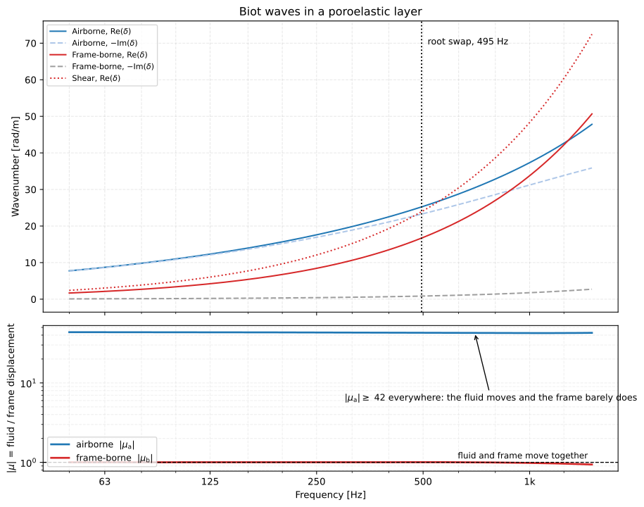
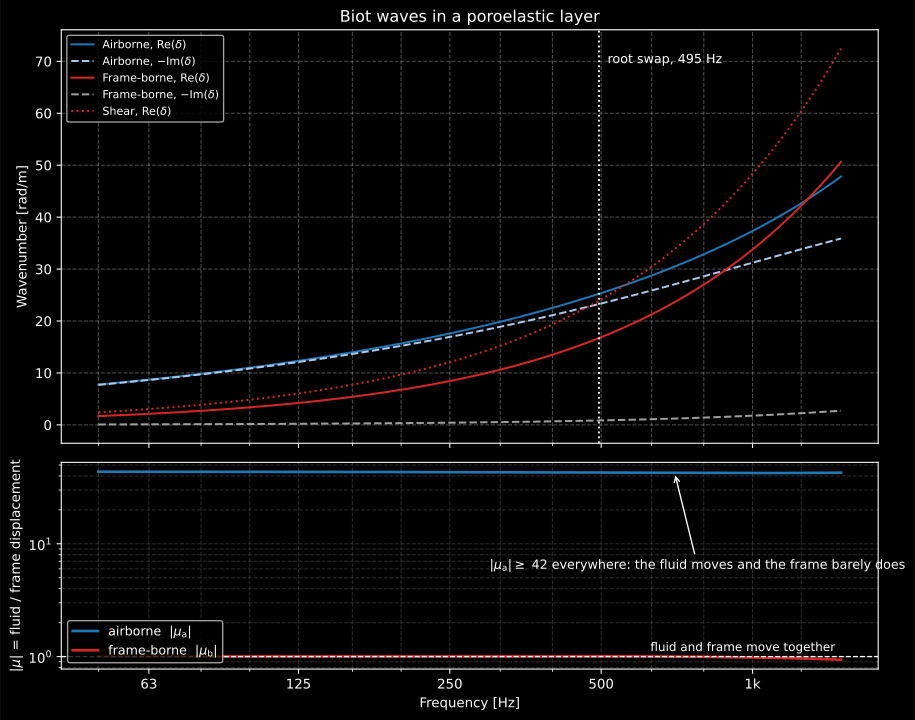
The three waves the Biot theory predicts where an equivalent fluid predicts one, for the Allard & Atalla Table 6.1 glass wool. The lower panel is what names them: $|{\mu }_a|$ never falls below 42, so in the airborne wave the pore fluid moves and the frame barely does — that is the wave the equivalent-fluid models already describe. $|{\mu }_b|$ sits on 1, so in the frame-borne wave fluid and frame move together, and no equivalent fluid has such a branch at all. The dotted line at 495 Hz is where the solver’s two compressional roots exchange places; the labelling follows $|\mu |$, not the eigenvalue order, so the curves stay continuous across it.

Show the code for this figure

# The BiotWavesResult of the Table 6.1 glass wool. Its .plot() draws the upper
# panel; the lower one is two of its fields.
f_biot = np.linspace(50.0, 1500.0, 1451)
biot = materials.biot_waves(
    materials.johnson_champoux_allard(
        f_biot, 40e3, porosity=0.94, tortuosity=1.06,
        viscous_length=0.56e-4, thermal_length=1.1e-4,
    ),
    porosity=0.94, tortuosity=1.06, frame_density=130.0,
    shear_modulus=2.2e6 * (1 + 0.1j),
)
print(round(float(abs(biot.airborne_velocity_ratio).min()), 1))    # 42.4
print(round(float(abs(biot.frame_borne_velocity_ratio[0])), 3))    # 1.002

biot_waves takes the rigid-frame equivalent fluid of the pores, normally a johnson_champoux_allard result. That is deliberate: the frame inertia is the Biot model’s own business, so handing it a limp_frame medium would count that inertia twice.

The consequence a designer cares about is a resonance. A layer glued to a rigid wall holds its frame still at the wall and free at the front face, so the frame-borne wave resonates a quarter wavelength inside the layer, at

$$f_r=\frac{1}{4l}\sqrt{\frac{\mathrm{Re}(K_c)}{{\rho }_1}},K_c=\frac{2(1-\nu )N}{1-2\nu }$$

(Eqs. 6.109-6.111), where $K_c$ is the longitudinal elastic coefficient of the frame in vacuum and ${\rho }_1$ its bulk density. frame_quarter_wave_resonance evaluates it. Nothing in the rigid-frame or limp-frame models can produce that peak.

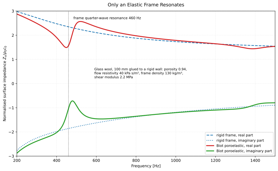
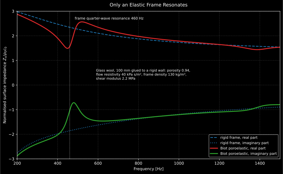
The glass wool of Allard & Atalla Table 6.1, 100 mm glued to a rigid wall, under both models. Away from the resonance the two are indistinguishable, which is the plot’s own check on the Biot layer; around it the poroelastic prediction develops the dip-and-peak in the real part and the sharp maximum in the imaginary part that the book measures and plots in its Fig. 6.10.

Show the code for this figure

import matplotlib.pyplot as plt
import numpy as np
from phonometry import (
    PoroelasticLayer, PorousLayer, biot_waves, frame_elastic_coefficient,
    frame_quarter_wave_resonance, johnson_champoux_allard, layered_absorber,
)

# Allard & Atalla Table 6.1: glass wool "Domisol Coffrage", 100 mm, glued.
f = np.linspace(200.0, 1500.0, 1301)
shear = 2.2e6 * (1 + 0.1j)          # 220 N/cm2, loss factor 0.1
med = johnson_champoux_allard(
    f, 40e3, porosity=0.94, tortuosity=1.06,
    viscous_length=0.56e-4, thermal_length=1.1e-4,
)

print(frame_elastic_coefficient(shear, 0.0))       # (4400000+440000j)
print(round(frame_quarter_wave_resonance(
    0.10, shear_modulus=shear, poisson_ratio=0.0, frame_density=130.0), 1))
# 459.9

waves = biot_waves(med, porosity=0.94, tortuosity=1.06,
                   frame_density=130.0, shear_modulus=shear)
print(round(float(abs(waves.airborne_velocity_ratio[800])), 1))     # 42.4
print(np.round(waves.frame_borne_velocity_ratio[-1], 3))  # (0.811+0.473j)

biot = layered_absorber(f, [PoroelasticLayer(0.10, med, 0.94, 1.06, 130.0, shear)])
rigid = layered_absorber(f, [PorousLayer(0.10, med)])

fig, ax = plt.subplots()
for res, style in ((rigid, "--"), (biot, "-")):
    ax.plot(f, res.normalized_impedance.real, style)
    ax.plot(f, res.normalized_impedance.imag, style)
ax.set(xlabel="Frequency [Hz]", ylabel="Zs / rho0 c0", ylim=(-3, 3))
plt.show()

waves.plot()   # the three Biot wavenumbers against frequency
plt.show()

Inside a stack, a PoroelasticLayer carries the same six variables the theory needs, $[v_1^s,v_3^s,v_3^f,{\sigma }_{33}^s,{\sigma }_{13}^s,{\sigma }_{33}^f]$, so layered_absorber switches from the two-variable chain to the global-matrix assembly of Allard & Atalla Sect. 11.5: fluid and sheet layers keep their 2x2 matrices, each poroelastic layer enters through the six wave amplitudes of its own $[\Gamma ]$ blocks rather than through a transfer matrix, and the two are joined by the printed coupling matrices of Sect. 11.4. Solving for the amplitudes directly avoids inverting $[\Gamma (0)]$, which is what makes a very soft or very thick frame tractable at all. Two adjacent poroelastic layers are coupled as bonded frames (their Eq. 11.67); a sheet next to one is coupled as a free, mechanically decoupled screen. The returned transfer_matrix is filled with nan for such a stack, because a 2x2 chain matrix does not exist for it; the surface impedance, reflection factor and absorption are unaffected.

For the same 100 mm layer the resonance moves absorption by up to 0.21 at its sharpest; on third-octave centres the largest shift is the 0.12 at 500 Hz:

import numpy as np
from phonometry import (
    PoroelasticLayer, PorousLayer, johnson_champoux_allard, layered_absorber,
)

bands = np.array([250, 315, 400, 500, 630, 800, 1000], dtype=float)
med = johnson_champoux_allard(
    bands, 40e3, porosity=0.94, tortuosity=1.06,
    viscous_length=0.56e-4, thermal_length=1.1e-4,
)
shear = 2.2e6 * (1 + 0.1j)
for layer in (PorousLayer(0.10, med),
              PoroelasticLayer(0.10, med, 0.94, 1.06, 130.0, shear)):
    print(layered_absorber(bands, [layer]).absorption.round(2))
# [0.55 0.58 0.62 0.65 0.69 0.74 0.78]   rigid frame
# [0.53 0.56 0.61 0.77 0.71 0.74 0.78]   Biot poroelastic

The layer is worth the extra five parameters when the frame is stiff and heavy enough to resonate in the band of interest (dense mineral wool, structural foams), when the material is bonded to a plate that shakes it directly, or when a measured impedance shows a feature no equivalent fluid can explain. A light, soft blanket in free air is better served by limp_frame.

Honest note on validation. There is no published table of $Z_s(f)$ or $\alpha (f)$ for a fully specified Biot layer, here or anywhere else checked, so this model cannot be pinned digit by digit the way the standards-based modules are. What it is anchored on instead, in decreasing strength: the rigid-frame limit, where making the frame infinitely stiff and heavy must reproduce the JCA equivalent fluid, whose own conformance is pinned on published digits, and does so with a residual that falls exactly as the inverse of the stiffness over eight decades, at four angles of incidence, with and without a rigid backing; the limp limit, where taking the stiffness to zero reproduces limp_frame; the agreement to machine precision between the two independent derivations the book gives, the ch. 6 closed form Eq. 6.107 and the ch. 11 global-matrix assembly; and the three computed numbers the book does print in prose for the Table 6.1 glass wool, all reproduced: the airborne wave changes root at 495 Hz, $|{\mu }_a|>40$ above 50 Hz, and ${\mu }_b$ falls from 1.0 at 50 Hz to 0.82 at 1500 Hz. That last one is matched by $\mathrm{Re}({\mu }_b)$, not by $|{\mu }_b|$, even though the printed sentence says “the ratio modulus”: the model gives ${\mu }_b(1500)=0.811+0.473j$, whose real part is 1.1 % from the printed value while its modulus, 0.939, is 14.5 % away. That is recorded in Errata, along with the parameter sweep that fails to bring $|{\mu }_b|$ anywhere near 0.82. The impedance peak of the book’s thinner sample is printed as 860 Hz and comes out at 863.5 Hz under the $\mathrm{Im}(Z_s)$ peak rule. Everything else, including the whole oblique-incidence behaviour beyond its rigid-frame limit, rests on closed forms and on structural identities, not on published digits.

2. Multilayer prediction by transfer matrices

Each fluid layer of thickness $d$ contributes the chain matrix (Cox & D’Antonio Eq. 2.29; equivalently the impedance recursion of Bies Eq. D.95 and Mechel Sect. D.4)

$${\left[\begin{array}{c}p\\ u\end{array}\right]}_{\text{front}}=\left[\begin{array}{cc}\cos (k_{x}d)& j{Z}_x\sin (k_{x}d)\\ j\sin (k_{x}d)/Z_x& \cos (k_{x}d)\end{array}\right]{\left[\begin{array}{c}p\\ u\end{array}\right]}_{\text{back}},$$

with the in-depth wavenumber $k_x=\sqrt{k^2-k_0^2{\sin }^2\theta }$ from Snell’s law and $Z_x=Z_{c}k/k_x$. Thin resonant sheets enter as series impedances $[[1,z],[0,1]]$. Closing the chain with a rigid wall (or free air, or any impedance) gives the surface impedance, the reflection factor $R(\theta )$ and $\alpha (\theta )=1-|R{|}^2$. A single hard-backed porous layer reduces to the textbook closed form $Z_s=-j{Z}_c\cot (kd)$ (Mechel Sect. D.3, Eq. 1).

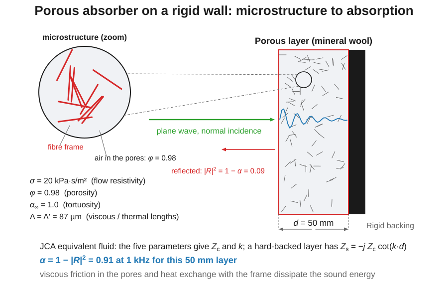
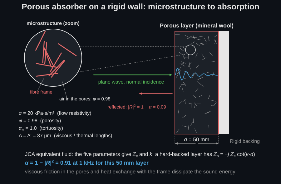
Behind the matrices there is one physical picture: a hard-backed porous layer is an equivalent fluid wrapped in five measurable numbers. The 50 mm layer below, evaluated with the five-parameter JCA model those numbers belong to, absorbs 91 % of a normal-incidence 1 kHz wave; the code that follows runs the same layer through the one-parameter Miki fit instead, which lands slightly higher (0.937), a fair picture of the spread between the two models.

import numpy as np
from phonometry import materials

f = np.geomspace(200.0, 4000.0, 300)
med = materials.miki(f, 20000.0)
res = materials.layered_absorber(f, [materials.PorousLayer(0.05, med)])
i = np.argmin(np.abs(f - 1000.0))
print(round(res.absorption[i], 3))               # 0.937 at 1 kHz

res.plot()   # alpha(f) with |R| overlaid

Spacing the layer off the wall. The commonest move in absorber design is not more material, it is a cavity, and the reason is in the boundary condition. A porous layer dissipates through the particle velocity in its pores, and a rigid backing forces that velocity to zero at the wall — so a layer thin against the wavelength sits in the dead zone and does almost nothing at low frequency. Move it back by $d$ and it sits near the velocity maximum at the frequency where the cavity is a quarter wavelength, $c_0/4d$, which is 858 Hz for a 100 mm gap (the layer’s own presence pulls the useful gain lower still). The arithmetic is worth seeing:

# The same 50 mm blanket, hard against the wall and spaced off it.
bands_gap = np.array([125.0, 250.0, 500.0, 1000.0])
med_gap = materials.miki(bands_gap, 20000.0)
flat = materials.layered_absorber(bands_gap, [materials.PorousLayer(0.05, med_gap)])
spaced = materials.layered_absorber(
    bands_gap, [materials.PorousLayer(0.05, med_gap), materials.AirLayer(0.10)]
)
thick = materials.layered_absorber(bands_gap, [materials.PorousLayer(0.15, med_gap)])
print(np.round(flat.absorption, 2))     # [0.09 0.26 0.62 0.94]  50 mm on the wall
print(np.round(spaced.absorption, 2))   # [0.44 0.78 0.9  0.77]  50 mm + 100 mm gap
print(np.round(thick.absorption, 2))    # [0.52 0.71 0.8  0.89]  150 mm on the wall

At 250 Hz the 50 mm layer on a 100 mm cavity beats 150 mm of solid blanket — 0.78 against 0.71 — for a third of the material and the same 150 mm of total depth. Two limits come with the trick: the gain disappears above the first cavity half-wave, where the layer lands back in a velocity node (visible as the spaced curve falling below the flat one at 1 kHz), and on a large surface the cavity must be partitioned or the field propagates laterally inside it at oblique incidence. This is the prediction counterpart of ISO 354’s Type E-xxx and G-xxx mountings, whose suffix is exactly this $d$.

The solver evaluates the physical quantities through a numerically robust admittance recursion (immune to the $e^{|\mathrm{Im}(k_x)|d}$ overflow of raw matrix entries for extremely attenuating layers) and still exposes the full chain matrix (reciprocal by construction, $\det T=1$) in transfer_matrix, ready for the ASTM E2611 machinery (TransferMatrix).

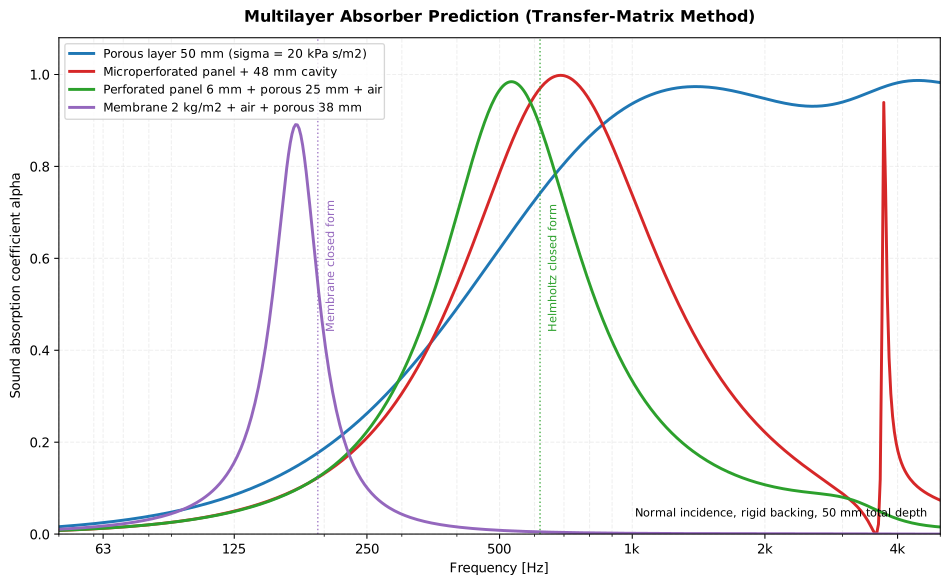
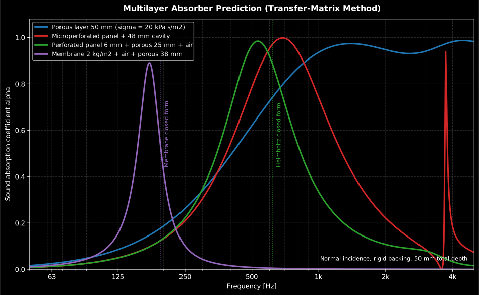
Four constructions, one 50 mm budget: the porous layer works broadband but fades at low frequency; the microperforated, perforated and membrane designs trade bandwidth for a resonant peak placed ever lower. The dotted lines are the shallow-cavity closed forms; the full model sits below them because the viscous plug mass and the finite cavity depth are not negligible.

Show the code for this figure

import matplotlib.pyplot as plt
import numpy as np
from phonometry import materials as m

f = np.geomspace(50.0, 5000.0, 500)
med = m.miki(f, 20000.0)
med_light = m.miki(f, 10000.0)
designs = {
    "Porous 50 mm": [m.PorousLayer(0.05, med)],
    "MPP + cavity": [m.MicroperforatedPlateLayer(0.5e-3, 0.15e-3, 0.008),
                     m.AirLayer(0.048)],
    "Perforated + porous": [m.PerforatedPlateLayer(0.006, 0.0025, 0.05),
                            m.PorousLayer(0.025, med), m.AirLayer(0.019)],
    "Membrane + porous": [m.MembraneLayer(2.0), m.AirLayer(0.01),
                          m.PorousLayer(0.038, med_light)],
}
fig, ax = plt.subplots()
for label, layers in designs.items():
    ax.semilogx(f, m.layered_absorber(f, layers).absorption, label=label)
ax.set(xlabel="Frequency [Hz]", ylabel="Absorption coefficient")
ax.legend()
plt.show()

Behind every one of those curves there is a plain layer list, read front to back in the order the incident wave meets it. plot_absorber_stack draws that list to scale before any physics runs, and a solved result retains its layers, so materials.layered_absorber(f, layers).plot_geometry() draws the same cross-section from the result itself.

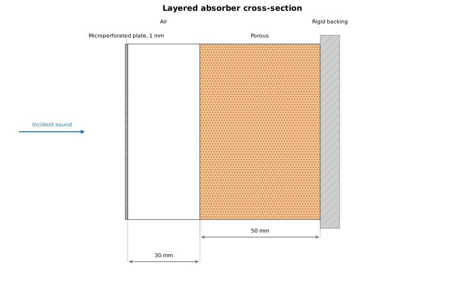
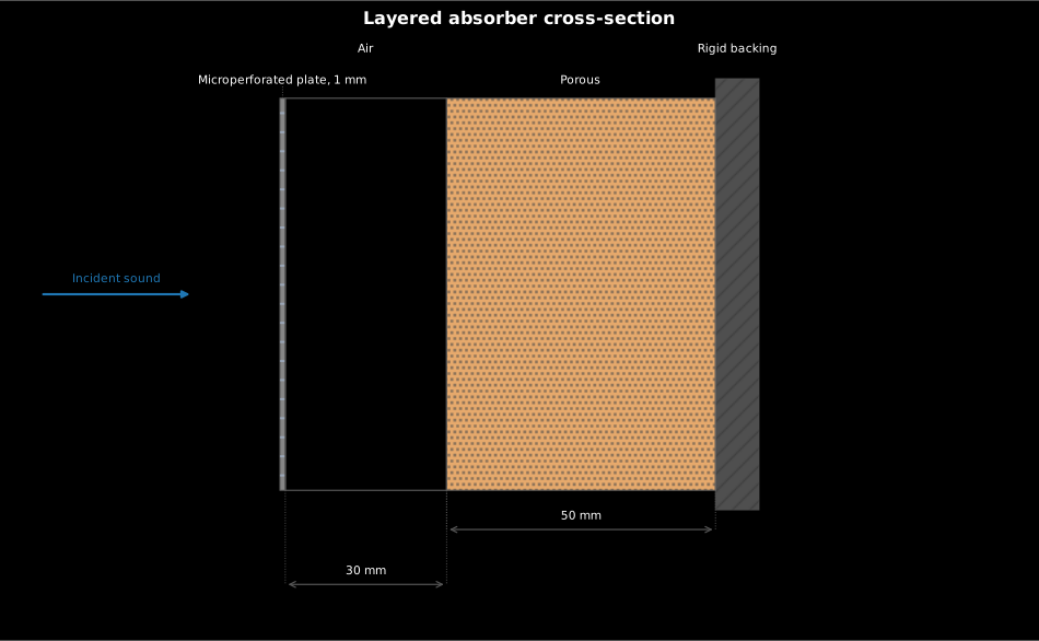
The layer list as the wave meets it: microperforated plate, air cavity, porous layer, rigid backing. Drawing the stack to scale before computing anything catches the classic metres-versus-millimetres slip in a thickness at a glance.

Show the code for this figure

import matplotlib.pyplot as plt
import numpy as np
from phonometry import materials

f = np.linspace(200.0, 4000.0, 100)
layers = [
    materials.MicroperforatedPlateLayer(0.001, 0.0002, 0.01),
    materials.AirLayer(0.03),
    materials.PorousLayer(0.05, materials.miki(f, 20000.0)),
]

# The free function draws any layer list; a solved result retains its
# layers, so this draws the same cross-section:
#   materials.layered_absorber(f, layers).plot_geometry()
materials.plot_absorber_stack(layers)
plt.show()

3. Resonant sheets: perforated, microperforated, membrane

Perforated panel. The air plugs in the holes are the mass of a Helmholtz resonator: $m=({\rho }_0/\epsilon )[t+2\delta a+\sqrt{8\nu /\omega }(1+t/2a)]$ with the open area $\epsilon$, the end-correction factor $\delta$ per orifice end and the visco-thermal resistance $r=({\rho }_0/\epsilon )\sqrt{8\nu \omega }(1+t/2a)$ (Cox & D’Antonio Eqs. 7.6/7.12). The default end correction is the Fok-function interaction fit $\delta =0.85(1-1.47\sqrt{\epsilon }+0.47{\epsilon }^{3/2})$ (Table 7.1), valid for any open area. For a shallow cavity the resonance is $f_0=(c_0/2\pi )\sqrt{\epsilon /(t^{\prime }d)}$ (Eq. 7.4). In those two expressions $t$ is the plate thickness, $a$ the hole radius, $\epsilon$ the open area (hole area over panel area), $\nu$ the kinematic viscosity of air, $t^{\prime }=t+2\delta a$ the end-corrected plate thickness and $d$ the cavity depth behind the panel.

Why a perforated panel needs porous material behind it. The resonance formula places the peak; the resistance decides its height and its width, and that is where an ordinary perforated panel is weak. Its holes are millimetres across, so the viscous loss in each plug is a small fraction of ${\rho }_0{c}_0$: over an empty cavity the construction is a high-Q resonator that absorbs over a narrow band and does almost nothing elsewhere. The standard fix is to put the missing resistance in the cavity — a porous layer or a resistive fleece — which lowers and broadens the peak towards the matched condition. That is exactly why the “Perforated + porous” design in the figure above carries a PorousLayer behind the plate, and why the MPP below can do without one: its sub-millimetre holes supply the resistance themselves. Two design consequences follow: place the porous layer where the particle velocity is high, which means against the perforated plate rather than flat on the rigid backing, and aim for a total flow resistance of the order of ${\rho }_0{c}_0$. The same statement read as an impedance match is the critical-coupling condition of the metamaterial guide.

The sheet layer classes: parameters

The three sheet layers take positional arguments, and the hole dimension is a radius, not a diameter — half the drilled hole. Getting that wrong computes the resonance and the peak absorption for a hole twice the real size.

Class	Parameter	Units	Notes
PerforatedPlateLayer	thickness	m	Plate thickness $t$
	hole_radius	m	Hole radius $a$, half the drilled diameter
	open_area	—	Perforation ratio $\epsilon$ = hole area / panel area
	end_correction	—	$\delta$ per orifice end; None uses the Fok interaction fit
MicroperforatedPlateLayer	thickness	m	Plate thickness $t$
	hole_radius	m	Hole radius $a$
	open_area	—	Perforation ratio $\epsilon$
	end_correction	—	Default 0.85, Maa’s piston reactance
MembraneLayer	surface_density	kg/m²	Mass per unit area $m$
	resistance	Pa·s/m	Added flow resistance; default 0.0

Microperforated panel (MPP). With submillimetre holes the viscous boundary layer fills the orifice and the panel absorbs without any porous material. The library implements Maa’s exact short-tube impedance (Maa 1998, Eq. 2),

$$z_1=j\omega {\rho }_{0}t{\left[1-\frac{2}{x\sqrt{-j}}\frac{J_1(x\sqrt{-j})}{J_0(x\sqrt{-j})}\right]}^{-1},x=a\sqrt{{\rho }_0\omega /\eta },$$

plus the Eq. 5 end corrections (surface resistance $\frac{1}{2}\sqrt{2\omega {\rho }_0\eta }$ and piston reactance $0.85d$ total), divided by the open area. The perforate constant $x$ (proportional to the hole radius over the viscous boundary-layer thickness) governs everything: at the resonance ${\omega }_{0}m=\cot ({\omega }_{0}D/c_0)$ the peak absorption is $4r/(1+r{)}^2$ and the half-absorption bandwidth is $f_2/f_1=\pi /\mathrm{arccot}(1+r)-1$ (Maa Eqs. 9–21, Table I).

import numpy as np
from phonometry import materials

# Maa (1998) Fig. 5: hole diameter 0.2 mm (so hole_radius = 0.1 mm),
# plate 0.2 mm thick, holes every 2.5 mm, cavity 6 cm.
eps = (np.pi / 4.0) * (0.2 / 2.5) ** 2
f = np.linspace(100.0, 4000.0, 2000)
res = materials.layered_absorber(
    f, [materials.MicroperforatedPlateLayer(0.2e-3, 0.1e-3, eps),
        materials.AirLayer(0.06)],
)
i = np.argmax(res.absorption)
print(f"peak alpha = {res.absorption[i]:.2f} at {f[i]:.0f} Hz")
# peak alpha = 0.96 at 677 Hz
res.plot()   # alpha(f) with |R| overlaid: the resonant MPP peak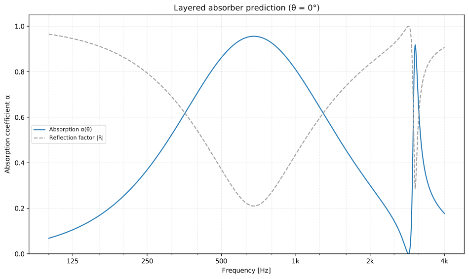

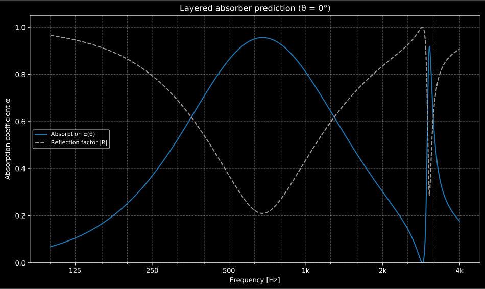
Maa’s own Fig. 5 design, no porous material anywhere: the viscous losses in the submillimetre holes damp the panel-cavity resonance into a broad absorption peak. The narrow feature near 2.9 kHz is the half-wave cavity resonance, where the cavity presents a pressure node to the panel and the absorption collapses before the next resonance restores it.

Show the code for this figure

import matplotlib.pyplot as plt
import numpy as np
from phonometry import materials

# Maa (1998) Fig. 5: hole diameter 0.2 mm (so hole_radius = 0.1 mm),
# plate 0.2 mm thick, holes every 2.5 mm, cavity 6 cm.
eps = (np.pi / 4.0) * (0.2 / 2.5) ** 2
f = np.linspace(100.0, 4000.0, 1200)
res = materials.layered_absorber(
    f, [materials.MicroperforatedPlateLayer(0.2e-3, 0.1e-3, eps),
        materials.AirLayer(0.06)],
)

# One line: alpha(f) with |R| overlaid.
res.plot()
plt.show()

# By hand, from the result's fields:
fig, ax = plt.subplots()
ax.semilogx(f, res.absorption, label="Absorption alpha")
ax.semilogx(f, np.abs(res.reflection), "--", label="Reflection factor |R|")
ax.set(xlabel="Frequency [Hz]", ylabel="Coefficient")
ax.legend()
plt.show()

Membrane. A limp impervious sheet is the surface mass $z=j\omega m$ (Cox Eq. 7.14; Bies Eq. D.96); over a cavity it resonates at the classical $f_0\approx 60/\sqrt{md}$ (adiabatic; $\approx 50/\sqrt{md}$ when the cavity is porous-filled and isothermal, Cox Eqs. 7.9/7.10). The closed forms are exposed as helmholtz_resonance_frequency and membrane_resonance_frequency; the full frequency response comes from the same layer stack.

The sheet impedance itself

The layer classes above hand their transfer impedance to the multilayer solver, and the solver gives back $\alpha (f)$ — which is how a resonant sheet is evaluated, not how it is designed. Every design relation in this section is written in $r$ and $\omega m$, so the same impedances are exposed on their own: perforated_plate_impedance, microperforated_plate_impedance and membrane_impedance, all returning $z$ in Pa·s/m before normalisation, plus perforation_end_correction for the Fok factor. With them the design argument closes on itself — the reactance crosses the cavity’s $-\cot (\omega D/c_0)$ at the resonance, and the resistance there fixes both the peak height $4r/(1+r{)}^2$ and the bandwidth:

# Maa's own Fig. 5 geometry, read as an impedance at its 677.5 Hz peak.
rho_c = 1.205 * 343.0
f_peak = np.array([677.5])
z_mpp = materials.microperforated_plate_impedance(
    f_peak, thickness=0.2e-3, hole_radius=0.1e-3, open_area=eps
)
r_mpp = float(z_mpp.real[0]) / rho_c
print(round(r_mpp, 3), round(float(z_mpp.imag[0]) / rho_c, 3))   # 1.531 1.077
print(round(4 * r_mpp / (1 + r_mpp) ** 2, 3))    # 0.956 = the peak alpha above

# The same panel with millimetre holes instead: an order of magnitude less
# resistance, hence the narrow peak that needs porous backing.
z_perf = materials.perforated_plate_impedance(
    f_peak, thickness=0.006, hole_radius=0.0025, open_area=0.05
)
print(round(float(z_perf.real[0]) / rho_c, 4))   # 0.0925, 16x lower

# A membrane is pure reactance unless a fixing resistance is supplied.
print(np.round(materials.membrane_impedance(f_peak, surface_density=2.0), 1))
# [0.+8513.6j]

# The Fok interaction: crowded holes shorten the effective plug.
print(round(materials.perforation_end_correction(0.05), 3))   # 0.575 vs 0.85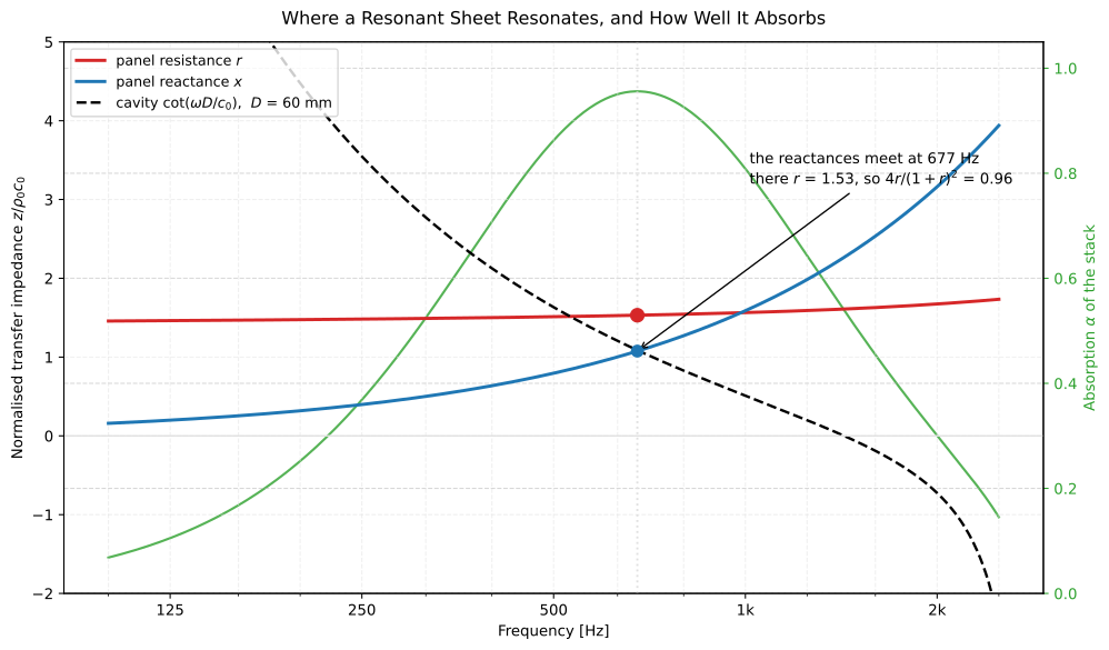

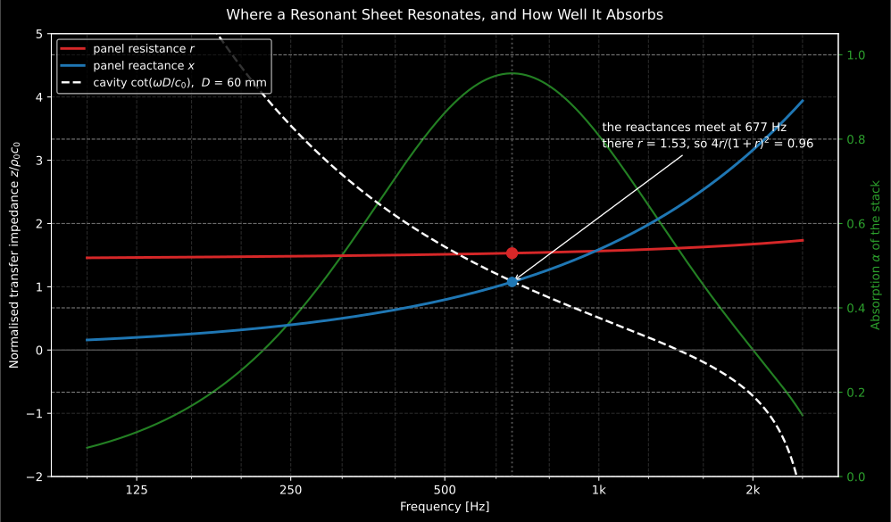
The whole design rule of this section in one picture. The panel reactance $x(f)$ and the cavity reactance $-\cot (\omega D/c_0)$ cross at 677 Hz: that crossing is the resonance, and it is placed by the geometry. What happens at the crossing is set by the resistance there, $r=1.53$, which gives $4r/(1+r{)}^2=0.96$ — the peak the stack computes, recovered from two numbers. A panel with millimetre holes has $r$ sixteen times smaller, so its crossing would be just as sharp and far less absorbent, which is the whole argument for either sub-millimetre holes or porous backing.

Show the code for this figure

f_sheet = np.geomspace(100.0, 4000.0, 400)
z_sheet = materials.microperforated_plate_impedance(
    f_sheet, thickness=0.2e-3, hole_radius=0.1e-3, open_area=eps
) / rho_c
cavity = -1.0 / np.tan(2.0 * np.pi * f_sheet * 0.06 / 343.0)
print(round(float(z_sheet.real[0]), 2), round(float(cavity[0]), 2))

Building what the stack predicts

The transfer-matrix stack assumes an infinite, laterally uniform, locally reacting construction. Five things have to be true on site for that assumption to survive.

1. Partition or fill the cavity behind a resonant facing. The one-dimensional model and the local-reaction assumption both need cells small against the wavelength at the design frequency. An unpartitioned cavity behind a perforated facing lets the field propagate laterally, which turns a locally reacting design into a bulk-reacting one and typically broadens and lowers the peak.
2. Seal the perimeter to the substrate, or the cavity is vented and the resonance it was tuned for does not exist.
3. Check the open area against the sheet you actually bought. The model’s $\epsilon$ is the geometric ratio $(\pi /4)(d_{\text{hole}}/b{)}^2$ for holes of diameter $d_{\text{hole}}$ on a pitch $b$. Burrs, paint and partly blocked sub-millimetre holes move the MPP resistance directly, and the resistance is what the peak height depends on.
4. Mount a membrane limp and unstressed. Clamping and stiffening add a restoring force the $z=j\omega m$ model does not have, and push $f_0$ above the $60/\sqrt{md}$ estimate.
5. Do not assume the backing. The drawn stack ends on a rigid wall; a construction on a resilient substrate needs that backing impedance passed explicitly through termination= rather than left at "rigid".

4. Oblique and random incidence

layered_absorber(..., angle=theta) evaluates the full bulk-reacting stack at any polar angle; sheets are locally reacting (angle-independent), fluid layers refract per Snell’s law; for an MPP over a cavity this reproduces Maa’s oblique closed form (Eq. 23) exactly. The random-incidence coefficient is the Paris integral (Mechel Sect. D.5, Eq. 9)

$${\alpha }_{dif}=\frac{2}{{\sin }^2{\theta }_{lim}}{\int }_0^{{\theta }_{lim}}\alpha (\theta )\cos \theta \sin \theta \mathrm{d}\theta ,$$

evaluated by Gauss–Legendre quadrature in diffuse_field_absorption (angle_limit defaults to 90°; truncations at 75–87° are in use). That truncation is not decoration and deserves a decision rule. The integrand weights oblique angles most heavily, and it is precisely near grazing incidence that the infinite-plane theory stops describing a real test: a finite mounted specimen does not behave like an unbounded layer at 85°, and a diffuse field over a 10–12 m² sample simply does not deliver the grazing energy the full integral assumes, so the untruncated result tends to sit below measured values. What practitioners do follows: truncate around 78° when the intention is to compare with a reverberation-room measurement, and keep 90° when the intention is the theoretical random-incidence coefficient of an infinite surface. A truncated ${\alpha }_{dif}$ is a fitted engineering quantity rather than a physical one, so the limit must be quoted with the number — the snippet below prints the size of the decision. For a locally reacting surface with known normalised impedance the integral has the closed form of Mechel Eq. 10, exposed as statistical_absorption; its maximum over all passive impedances is the published 0.951 (at $z\approx 1.57$).

import numpy as np
from phonometry import materials

f = np.array([250.0, 500.0, 1000.0, 2000.0])
med = materials.miki(f, 20000.0)
layers = [materials.PorousLayer(0.05, med)]
normal = materials.layered_absorber(f, layers)
diffuse = materials.diffuse_field_absorption(f, layers)
print(np.round(normal.absorption, 2))    # [0.26 0.62 0.94 0.95]
print(np.round(diffuse.absorption, 2))   # [0.37 0.68 0.9  0.95]
diffuse.plot()   # alpha_dif(f); overlay normal.absorption to compare

print(round(float(materials.statistical_absorption(1.567 + 0j)), 3))  # 0.951

# What the truncation is worth, on the same layer.
truncated = materials.diffuse_field_absorption(f, layers, angle_limit=np.radians(78.0))
print(np.round(truncated.absorption - diffuse.absorption, 3))
# [-0.001  0.01   0.019  0.018]  a few hundredths, and it goes the right way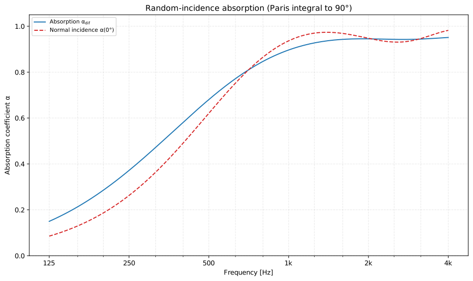

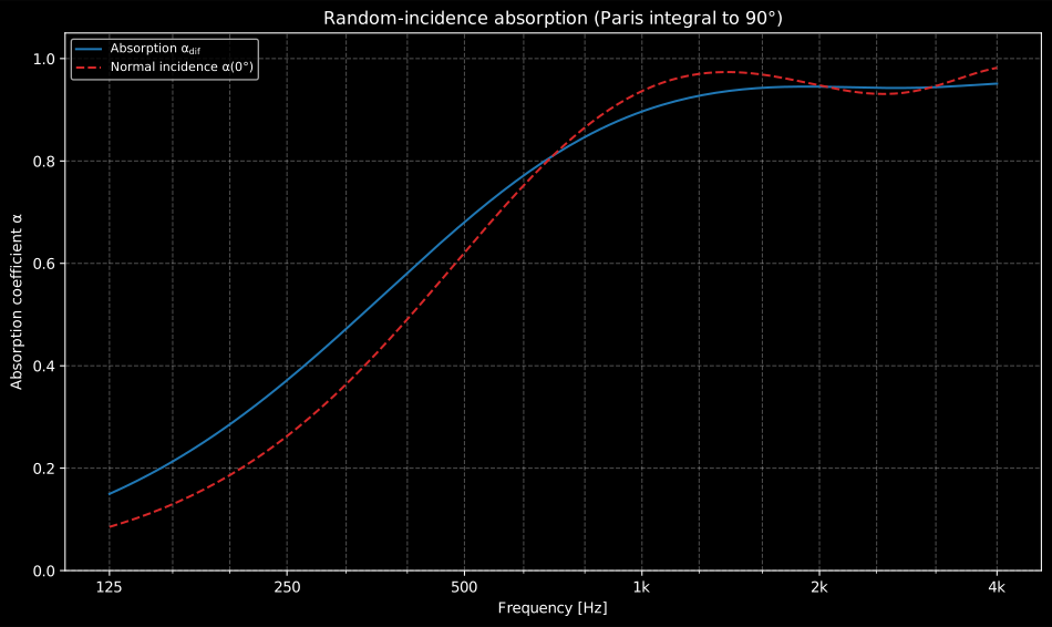
Why the reverberation room reads higher than the tube: the Paris integral weights the oblique angles, whose waves travel a longer path inside the layer, so ${\alpha }_{dif}$ exceeds the normal-incidence $\alpha (0°)$ exactly where the layer is thin against the wavelength. This is the model-side counterpart of the tube-versus-reverberation-room discussion of Sound Absorption Measurement and Rating.

Show the code for this figure

import matplotlib.pyplot as plt
import numpy as np
from phonometry import materials

f = np.geomspace(125.0, 4000.0, 200)
layers = [materials.PorousLayer(0.05, materials.miki(f, 20000.0))]
normal = materials.layered_absorber(f, layers)
diffuse = materials.diffuse_field_absorption(f, layers)

# One line, then the normal-incidence overlay on the same axes:
ax = diffuse.plot()
ax.plot(f, normal.absorption, "--", label="Normal incidence alpha(0)")
ax.legend()
plt.show()

Do not compare this with a datasheet ${\alpha }_s$. The Paris integral is evaluated on an infinite, laterally uniform layer. An ISO 354 measurement is made on a mounted 10–12 m² specimen whose edges diffract energy into it, which is why measured ${\alpha }_s$ routinely exceeds 1 and why the same product differs between two rooms. Expect the measured value to run above the predicted ${\alpha }_{dif}$ by roughly 0.1 to 0.2 in the mid bands, more as the specimen shrinks and its perimeter-to-area ratio rises. The corollary for model fitting is the important half: fit material parameters against a tube measurement, or against the diffuse prediction of a model you trust, and never against a datasheet ${\alpha }_s$ — the finite-size surplus would be absorbed into a wrong flow resistivity and then propagate into every construction you predict from it. What the prediction is good for is comparing constructions, sizing a treatment before it exists, and feeding a room calculation that expects random-incidence input; a specification written against a measured ${\alpha }_s$ still has to be closed with a measurement.

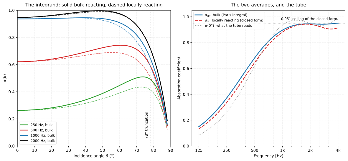
The integrand the Paris average consumes, and the two ways of averaging it. Left: $\alpha (\theta )$ of the same 50 mm layer at four frequencies, each solid bulk-reacting curve (layered_absorber(..., angle=theta), in which the fluid layers refract) shadowed by the locally reacting curve obtained from the same normal-incidence surface impedance. The two agree at normal incidence by construction, separate through the 40°–75° range where the Paris integrand carries most of its weight — the bulk model absorbing more, because the wave refracts and travels further inside the layer — and converge again as both collapse towards zero at grazing. The choice of reaction model is therefore a choice about the part of the integral that matters most. Right: the two integrated results over frequency, with the 0.951 maximum of the locally reacting closed form drawn as a ceiling no passive impedance can pass.

Show the code for this figure

# alpha(theta) at one frequency, both ways.
theta = np.radians(np.linspace(0.0, 88.0, 60))
f_one = np.array([1000.0])
layers_one = [materials.PorousLayer(0.05, materials.miki(f_one, 20000.0))]
bulk = [float(materials.layered_absorber(f_one, layers_one, angle=float(t)).absorption[0])
        for t in theta]
z_normal = materials.layered_absorber(f_one, layers_one).normalized_impedance[0]
local = [1.0 - abs((z_normal * np.cos(t) - 1.0) / (z_normal * np.cos(t) + 1.0)) ** 2
         for t in theta]
print(round(bulk[0], 3), round(bulk[-1], 3))     # 0.937 0.161
print(round(local[0], 3), round(local[-1], 3))   # 0.937 0.138

The classical layers above absorb with bulk or with a quarter-wave cavity. Their resonant metamaterial relatives, rigid panels of sub-millimetre slits loaded by Helmholtz resonators that slow the sound and reach perfect absorption ($\alpha =1$) at critical coupling in panels only $\lambda /38$ deep, moved to their own guide: Metamaterial Absorbers covers the transfer-matrix model, the critical-coupling design solver and the FDTD cross-check of the meshed cell.

Practical notes

Fit ranges. Delany–Bazley warns (and extrapolates) outside $0.01<X<1$ and Miki outside $0.01<f/\sigma <1$; treat sub-range values as qualitative. JCA needs four extra parameters but behaves physically everywhere; with $\Lambda ={\Lambda }^{\prime }=\sqrt{8{\alpha }_{\infty }\eta /(\varphi \sigma )}$ and ${\alpha }_{\infty }=1$ it tracks Delany–Bazley over the fit range.

Rigid or limp frame. Every equivalent-fluid model above assumes a motionless frame, which only holds above the decoupling frequency $F_d=\sigma {\varphi }^2/2\pi {\rho }_1$. Below it a light frame moves with the pore fluid, and limp_frame adds its inertia (Allard & Atalla Eqs 11.53-11.55). Use it for felts, screens and light fibreglass, for anything measured unconstrained in an impedance tube, and wherever the frame in vacuum is softer than about 20 kPa (limp_frame_applicable); do not use it, or the rigid model either, for a material bonded to a vibrating structure. When the frame is stiff and heavy enough to resonate in the band of interest, neither equivalent fluid will do at all: use a PoroelasticLayer and the full Biot theory.

Local vs. bulk reaction. The layer solver is bulk-reacting (sound refracts and travels inside the layers). statistical_absorption assumes local reaction, a good approximation for high flow resistivity, partitioned cavities or thin resonant facings; for thick, light porous layers integrate the bulk model with diffuse_field_absorption instead (Mechel Sect. D.6).

Where the numbers were checked. No standard governs these prediction models; they are textbook and journal methods implemented clean-room from the sources in the references below. The models are pinned digit-exact to the printed coefficient tables (Bies Table D.1, Miki Eqs. 30–34), the solver to the closed forms above and to the TransferMatrix recovery of the impedance-tube page, the MPP to Maa’s own approximation (stated ~6 % agreement with the exact Eq. 2), design example and Table I, and the Paris integral to its locally reacting closed form. Misprints found in the sources during this work are recorded in the errata registry.

What this guide covers

• Covered

  The textbook and journal methods of Mechel, Bies, Cox & D’Antonio, Miki (1990), Maa (1998) and Johnson, Koplik & Dashen (1987), implemented clean-room as described above, together with the Biot theory of Allard & Atalla chapters 6 and 11. That covers the equivalent-fluid porous models (delany_bazley, miki, johnson_champoux_allard, limp_frame), the poroelastic layer (biot_waves, biot_surface_impedance, PoroelasticLayer), the transfer-matrix multilayer solver (layered_absorber with AirLayer, PorousLayer, PoroelasticLayer, PerforatedPlateLayer, MicroperforatedPlateLayer and MembraneLayer) and the Paris-integral random-incidence coefficients (diffuse_field_absorption, statistical_absorption). The sheet transfer impedances the layer classes consume are also exposed on their own, which is how a resonant sheet is designed rather than merely evaluated: perforated_plate_impedance, microperforated_plate_impedance, membrane_impedance and perforation_end_correction.

• Not covered

  Nothing here measures anything: the five JCA parameters, the frame’s shear modulus and Poisson coefficient and the sheet geometry are all inputs, and section 1.1 says where they come from without implementing any of those characterisation methods (only the inverse fit against a measured impedance is shown, and that is scipy.optimize, not this library). The buildability rules at the end of section 3 are engineering practice with no standard behind them, and the finite-size difference between a predicted ${\alpha }_{dif}$ and a measured ${\alpha }_s$ is stated but not modelled — nothing here reproduces the edge effect. Cox & D’Antonio’s book covers diffusers as well as absorbers, but this guide only implements the absorber half of it. Schroeder phase-grating diffuser prediction lives in a separate module (materials.diffusers.design), documented in Diffusers and Their Coefficients and, for the resonator-loaded deep-subwavelength panels, in Metadiffusers. The critically coupled slit and Helmholtz-resonator absorber (slit_helmholtz_absorber, critical_coupling_design) is the subject of Metamaterial Absorbers.

See also

• Airflow Resistance, Impedance Tube and Sound Absorption Measurement and Rating: the measurement standards these prediction models connect to, namely ISO 9053-1/-2 (flow resistivity), ISO 10534-1/-2 and ASTM E2611 (impedance tube), and ISO 354 / ISO 11654 (random-incidence absorption and rating).
• Metamaterial Absorbers: the slow-sound slit panels and the critical-coupling condition that push perfect absorption into the deep-subwavelength regime.
• Theory: Acoustic material characterisation: the characterisation quantities the empirical and phenomenological models take as input.

References

• Allard, J. F., & Atalla, N. (2009). Propagation of Sound in Porous Media: Modelling Sound Absorbing Materials (2nd ed.). Wiley. https://doi.org/10.1002/9780470747339Chapter 6: the Biot theory of an elastic-framed porous material, its elastic coefficients, its two compressional waves and its shear wave, and the surface impedance and quarter-wave frame resonance of a hard-backed layer (Eqs 6.107-6.111). Chapter 11: the transfer-matrix method, the six-variable poroelastic layer matrix (Table 11.1), the coupling matrices (Sect. 11.4) and the global assembly (Sect. 11.5). Section 11.3.4: the rigid and limp frame limits of the Biot theory, the decoupling frequency and the limp effective density (Eqs 11.53-11.55, after Panneton 2007). ISBN 978-0-470-74661-5.
• Attenborough, K., & Van Renterghem, T. (2021). Predicting outdoor sound (2nd ed.). CRC Press. https://doi.org/10.1201/9780429470806Chapter 5: ground-impedance models, including the JCA family.
• Bies, D. A., Hansen, C. H., & Howard, C. Q. (2017). Engineering noise control (5th ed.). CRC Press. https://doi.org/10.1201/9781351228152Appendix D: porous-material properties, Table D.1 coefficient sets and the layered-construction recursions D.91-D.99.
• Cox, T. J., & D'Antonio, P. (2017). Acoustic absorbers and diffusers: Theory, design and application (3rd ed.). CRC Press. https://doi.org/10.1201/9781315369211Transfer-matrix modelling (Sect. 2.6), porous models (Sect. 6.5) and resonant-absorber design equations (Sects. 7.3/7.5).
• Delany, M. E., & Bazley, E. N. (1970). Acoustical properties of fibrous absorbent materials. Applied Acoustics, 3(2), 105-116. https://doi.org/10.1016/0003-682X(70)90031-9The original empirical relations and their stated validity.
• Hopkins, C. (2007). Sound insulation. Butterworth-Heinemann. https://doi.org/10.4324/9780080550473Section 1.3.2.2: the equivalent-gas model and the Delany-Bazley SI form.
• Johnson, D. L., Koplik, J., & Dashen, R. (1987). Theory of dynamic permeability and tortuosity in fluid-saturated porous media. Journal of Fluid Mechanics, 176, 379-402. https://doi.org/10.1017/S0022112087000727The dynamic-tortuosity model behind the JCA effective density.
• Maa, D.-Y. (1998). Potential of microperforated panel absorber. The Journal of the Acoustical Society of America, 104(5), 2861-2866. https://doi.org/10.1121/1.423870The exact MPP impedance (Eq. 2), end corrections, design formulas and the Fig. 5 example pinned in the tests.
• Mechel, F. P. (Ed.). (2008). Formulas of acoustics (2nd ed.). Springer. https://doi.org/10.1007/978-3-540-76833-3Sections D.3-D.6 (layer reflection, multilayer scheme, diffuse-field integrals) and G.11 (empirical porous relations).
• Miki, Y. (1990). Acoustical properties of porous materials — Modifications of Delany-Bazley models. Journal of the Acoustical Society of Japan (E), 11(1), 19-24. https://doi.org/10.1250/ast.11.19The positive-real regression implemented in miki.