Metamaterial Absorbers
Key references: Jiménez et al. 2017Jiménez et al. 2016Stinson 1991Maa 1998Cox & D'Antonio 2017Jiménez et al. 2021
A porous blanket absorbs low frequencies only by growing thick: the porous models put the useful absorption where the layer is a fair fraction of the wavelength, which at 300 Hz means tens of centimetres. Acoustic metamaterial absorbers break that rule with resonance instead of bulk. A rigid panel of thin closed slits, each loaded by Helmholtz resonators, slows the sound inside the slit so drastically that a 3 cm panel resonates at about 300 Hz, where an empty quarter-wave cavity would have to be ten times deeper, since 3 cm of plain air resonates at 2.9 kHz (section 3). Tuning the panel’s internal losses against its leakage then produces perfect absorption, , at a design frequency where the panel is only deep; published designs of the same family reach (Jiménez et al. 2016). This guide covers the critical-coupling condition that makes perfect absorption possible, the slow-sound slit panel implemented in the library, and the classical resonant absorbers re-read through the same lens.
1. Critical coupling: when loss exactly balances leakage
Section titled “1. Critical coupling: when loss exactly balances leakage”A rigidly backed absorber panel is a one-port resonator: sound enters through the face, rings inside, and either leaks back out or is dissipated. Its reflection coefficient over the complex frequency plane has a pole and a zero for each resonance. Two rates compete at the resonance: the leakage rate, how fast the stored energy radiates back into the incident medium, and the intrinsic loss rate, how fast the visco-thermal boundary layers of the structure dissipate it.
- Too little loss (an almost lossless panel) and the energy mostly leaks back out: the reflection dips but recovers, .
- Too much loss (an over-damped panel) and the wave barely enters: the panel starts to look rigid again, from the other side.
- When the two rates are equal, the zero of the reflection coefficient lands exactly on the real-frequency axis: at that frequency nothing is reflected, and . This is the critical-coupling condition (Jiménez et al. 2017).
In impedance terms the same statement reads : the panel’s surface
impedance is purely resistive and matched to the incident medium,
and . The condition says
nothing about thickness, which is exactly the loophole metamaterial absorbers
exploit: make the resonance deep-subwavelength with slow sound, then tune the
loss to match. The balance is delicate by design, and the library’s
critical_coupling_design solves it numerically rather than by trial: at the
returned geometry the normalised impedance sits at and the
reflection at zero.
Two lengths set the panel geometry and appear in every call below. The
lattice step lattice_step = is the spacing between successive
resonators along one slit, so a slit loaded by resonators is
deep: that, and not the resonator’s own cavity, is what makes the
panel 30 mm thick in the example. The period period_m = is the spacing
between slits across the panel face, so one slit of height serves each
period and the front face is referred to the cell area . The
resonator itself is described separately by its neck and cavity sides and
lengths.
import numpy as npfrom phonometry import materials
base = materials.HelmholtzResonator(    neck_length=1.0e-3, neck_side=3.0e-3,    cavity_length=30.0e-3, cavity_side=27.0e-3,)design = materials.critical_coupling_design(300.0, base, lattice_step=3.0e-2, period_m=5.0e-2)
f = np.array([300.0])res = materials.slit_helmholtz_absorber(    f, design.resonator, slit_height=design.slit_height,    lattice_step=3.0e-2, period_m=5.0e-2,)z = res.normalized_impedance[0]print(round(z.real, 2), round(z.imag, 2))       # 1.0 -0.0  (matched)print(round(float(np.abs(res.reflection[0])), 3))   # 0.0   (reflection zero)
Those two printed numbers are the whole of the evidence for the match, which is a pity, because the balance is easier to see than to read:
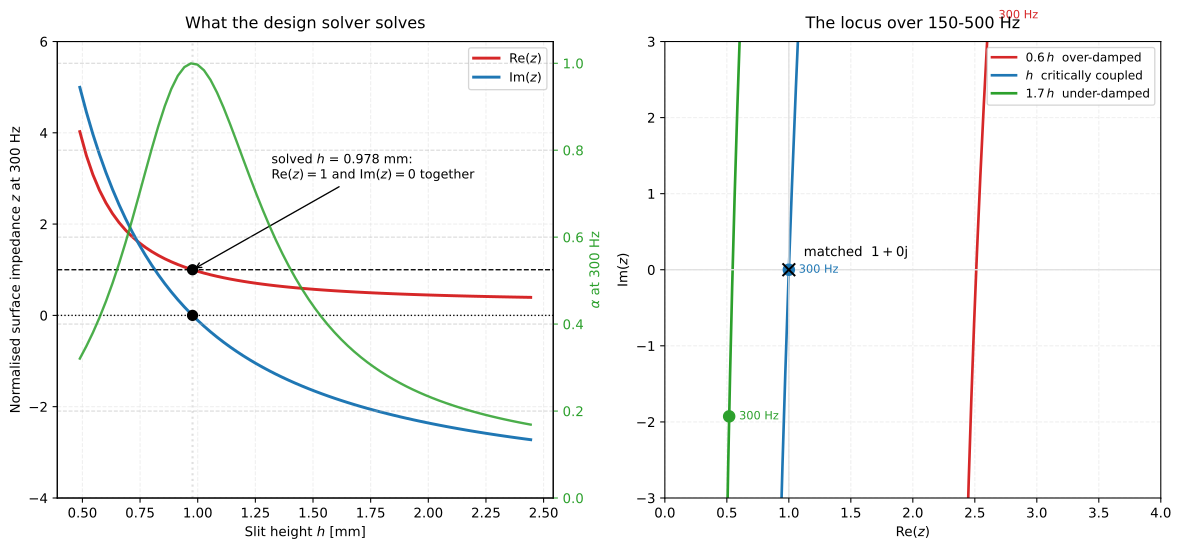
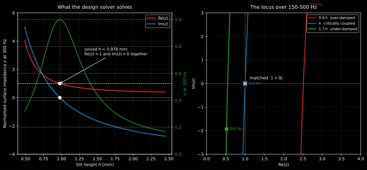
What critical_coupling_design is solving. Left: sweep the slit height at
the design frequency and the two matching conditions cross the same point,
and at 0.978 mm, where the
absorption reaches 1. Right: the same three slits as loci in the complex
plane. Over-damped and under-damped fail for opposite reasons, and the locus
says which side you are on; the absorption curve alone does not.
Show the code for this figure
# The impedance at 300 Hz as a function of slit height, in one line each.for factor in (0.6, 1.0, 1.7): z_h = materials.slit_helmholtz_absorber( np.array([300.0]), design.resonator, slit_height=factor * design.slit_height, lattice_step=3.0e-2, period_m=5.0e-2, ).normalized_impedance[0] print(factor, round(z_h.real, 2), round(z_h.imag, 2))# 0.6 2.61 3.34 over-damped: too resistive, and no longer resonant at 300 Hz# 1.0 1.0 -0.0 matched# 1.7 0.52 -1.93 under-damped: too little loss2. The slow-sound slit panel
Section titled “2. The slow-sound slit panel”A rigid panel perforated by a periodic array of thin closed slits, each slit loaded on its upper wall by an array of Helmholtz resonators, is a locally reacting, deep-subwavelength absorber (Jiménez et al. 2017). The resonators slow the sound inside the slit, pulling the slit resonance far below the quarter-wavelength frequency, so a panel a few centimetres deep resonates in the low hundreds of hertz. The visco-thermal losses in the sub-millimetre slit and in the resonator necks are what make perfect absorption possible: when the intrinsic loss exactly balances the leakage of the structure the reflection zero lands on the real-frequency axis and (critical coupling).
The panel transfer matrix is the chain of half-lattice slit steps (with slit characteristic impedance ), resonators as shunt point scatterers , and a slit-radiation end correction. The rigidly-backed reflection factor is with and . The slit uses the narrow-channel visco-thermal parameters and the square necks and cavities the rectangular-duct series of Stinson (1991).
Every symbol in that chain: is the half-lattice step of the slit itself, the shunt admittance of the -th resonator with its input impedance (neck plus cavity, with the radiation end corrections of Jiménez et al. 2016), and the radiation correction of the slit mouth. , and are the visco-thermal effective bulk modulus, effective density and cross-section of the slit. is the area of one period of the panel face, so is the section 1 matching impedance referred to that same area: the panel is matched when the sound entering one period is exactly consumed by it. Note the symbol does double duty: in section 1 is the medium impedance , here it is that impedance divided by a cross-section.
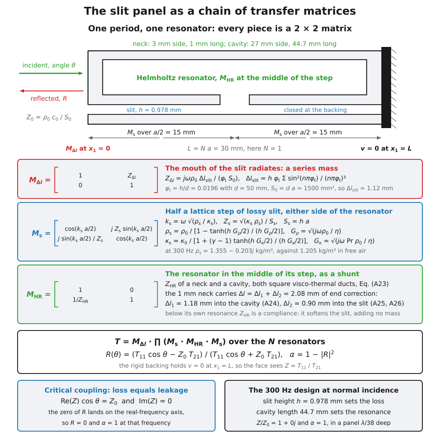
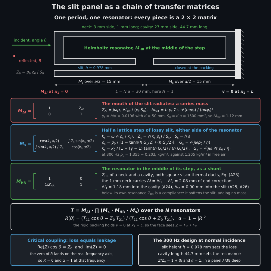
One period of the 300 Hz design as the chain the library multiplies: a radiation mass at the mouth, a lossy half step of slit either side of the resonator, the resonator as a shunt, and the rigid backing that turns the product into a surface impedance. Critical coupling is then two conditions on that impedance, and the design meets both with a 0.978 mm slit and a 44.7 mm cavity.
Watch what the solver actually changes. Given a target frequency it retunes the resonator’s cavity length and solves for the slit height; the lattice step and the period stay as passed. For the 300 Hz design below the cavity goes from the 30 mm of the starting resonator to 44.7 mm and the slit lands at 0.978 mm, while the panel stays 30 mm deep because mm, which is at 300 Hz. A reader who wants a deeper panel adds resonators, not cavity.
critical_coupling_design inverts the model: given a target frequency and
angle it tunes the cavity length (which sets the resonance) and the slit
height (which sets the loss) so both matching conditions
and hold, placing the
reflection zero on the real axis. The returned geometry then gives
at the design frequency.
import numpy as npfrom phonometry import materials
base = materials.HelmholtzResonator(    neck_length=1.0e-3, neck_side=3.0e-3,    cavity_length=30.0e-3, cavity_side=27.0e-3,)design = materials.critical_coupling_design(    300.0, base, lattice_step=3.0e-2, period_m=5.0e-2,)print(round(design.absorption, 4))          # ~1.0 (perfect absorption)print(round(design.slit_height * 1e3, 3))    # solved slit height, mm
f = np.linspace(150.0, 500.0, 700)res = materials.slit_helmholtz_absorber(    f, design.resonator, slit_height=design.slit_height,    lattice_step=3.0e-2, period_m=5.0e-2,)res.plot()   # alpha(f) with |R| overlaid; peak = 1 at 300 Hz
The solved geometry is worth a look before the absorption curve. The
resonator draws itself with .plot() and the panel result with
.plot_geometry(), both dimensioned and to scale.
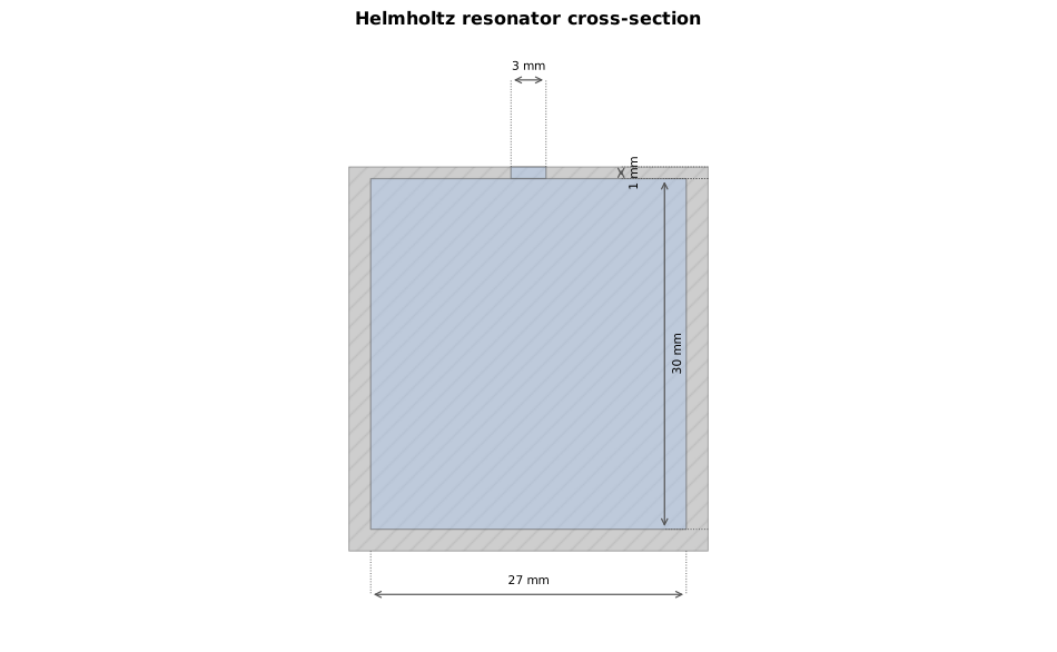
The four numbers that define the resonator: the neck side and length set
the moving mass and most of the loss, the cavity side and length set the
stiffness. critical_coupling_design keeps this cross-section and retunes
the cavity length to place the resonance.
Show the code for this figure
import matplotlib.pyplot as pltfrom phonometry import materials
resonator = materials.HelmholtzResonator(    neck_length=1.0e-3, neck_side=3.0e-3,    cavity_length=30.0e-3, cavity_side=27.0e-3,)resonator.plot()   # dimensioned cross-section, to scaleplt.show()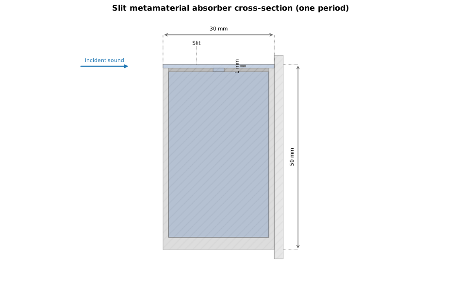
One period of the solved design, to scale: the whole panel is 30 mm deep, at 300 Hz, and the sub-millimetre slit that does all the absorbing is barely visible. That is exactly the point of the slow-sound mechanism.
Show the code for this figure
import matplotlib.pyplot as pltfrom phonometry import materials
base = materials.HelmholtzResonator(    neck_length=1.0e-3, neck_side=3.0e-3,    cavity_length=30.0e-3, cavity_side=27.0e-3,)design = materials.critical_coupling_design(    300.0, base, lattice_step=3.0e-2, period_m=5.0e-2,)
# The free function draws any resonator list; a slit_helmholtz_absorber# result retains its geometry, so res.plot_geometry() draws the same period_m.materials.plot_slit_absorber_geometry(    [design.resonator], slit_height=design.slit_height,    lattice_step=3.0e-2, period_m=5.0e-2,)plt.show()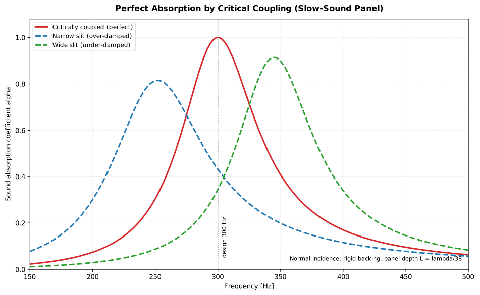
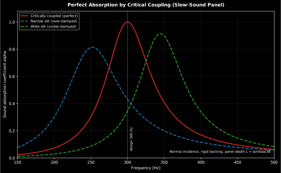
One resonator, one slit, one loss-versus-leakage balance. The critically coupled design reaches at 300 Hz in a panel only deep; narrowing the slit over-damps the resonance and widening it under-damps it, both dropping the peak below one.
Show the code for this figure
import matplotlib.pyplot as pltimport numpy as npfrom phonometry import materials
a, d, f0 = 3.0e-2, 5.0e-2, 300.0base = materials.HelmholtzResonator(1.0e-3, 3.0e-3, 30.0e-3, 27.0e-3)design = materials.critical_coupling_design(f0, base, lattice_step=a, period_m=d)h0 = design.slit_height
f = np.linspace(150.0, 500.0, 700)fig, ax = plt.subplots()for factor, label in [(1.0, "critically coupled"),                      (0.6, "narrow slit"), (1.7, "wide slit")]:    res = materials.slit_helmholtz_absorber(        f, design.resonator, slit_height=factor * h0,        lattice_step=a, period_m=d,    )    ax.plot(f, res.absorption, label=label)ax.set(xlabel="Frequency [Hz]", ylabel="Absorption coefficient")ax.legend()plt.show()
The clip below drives this exact cell in a virtual plane-wave tube: the sub-millimetre slit and its resonator are meshed on the FDTD grid and filled with the model’s visco-thermal effective fluids. At the design slit height the standing wave collapses and the tone dies inside the panel; at 1.7 times the height the loss balance breaks and the reflection rebuilds it.
A 300 Hz plane tone in a 2D FDTD tube meets the meshed critical-coupling cell, its 0.98 mm slit and Helmholtz resonator resolved on the grid and shown in a zoomed panel. At the design slit height the pressure envelope stays flat and the annotated library absorption is 1.00; the 1.7 times wider slit stands a deep wave in front of the panel and the absorption drops to 0.34.
A 300 Hz plane tone in a 2D FDTD tube meets the meshed critical-coupling cell, its 0.98 mm slit and Helmholtz resonator resolved on the grid and shown in a zoomed panel. At the design slit height the pressure envelope stays flat and the annotated library absorption is 1.00; the 1.7 times wider slit stands a deep wave in front of the panel and the absorption drops to 0.34.
Off normal incidence
Section titled “Off normal incidence”Every snippet and figure above is at normal incidence, and the matching condition carries a : . The structure is locally reacting, so the internal chain is angle-independent and only the front-face air impedance moves with ; a panel matched at normal incidence therefore becomes progressively mismatched as the angle grows, without the resonance moving in frequency. How much it costs is a question the model answers directly, and the answer is milder than the algebra suggests:
# The same 300 Hz design, evaluated off normal. Both the solver and the# evaluator take `angle_rad` in radians.for degrees in (0.0, 15.0, 30.0, 45.0, 60.0): off = materials.slit_helmholtz_absorber( np.array([300.0]), design.resonator, slit_height=design.slit_height, lattice_step=3.0e-2, period_m=5.0e-2, angle_rad=np.radians(degrees), ) print(degrees, round(float(off.absorption[0]), 3))# 0.0 1.0 / 15.0 1.0 / 30.0 0.995 / 45.0 0.971 / 60.0 0.889The peak stays at 300 Hz and falls only to 0.89 at 60°, which is what the
source paper means by quasi-omnidirectional absorption. Two design options
follow. Tune at the angle the panel will mostly see (critical_coupling_design
takes the same angle_rad argument) when the installation has a dominant
direction; or accept the normal-incidence design, which is the more tolerant
choice across angle. Either way, expect a
reverberation-room measurement of such a panel to come out below the
normal-incidence , since the diffuse field weights exactly the
oblique angles where the match is worst.
3. How slow is the sound?
Section titled “3. How slow is the sound?”The name of the mechanism is measurable. The transfer-matrix result retains the retrieved effective wavenumber of the loaded slit, so the phase speed inside it is one division away, and the comparison with the empty slit says everything about why the panel can be thin:
import numpy as npfrom phonometry import materials
base = materials.HelmholtzResonator(    neck_length=1.0e-3, neck_side=3.0e-3,    cavity_length=30.0e-3, cavity_side=27.0e-3,)design = materials.critical_coupling_design(300.0, base, lattice_step=3.0e-2, period_m=5.0e-2)res = materials.slit_helmholtz_absorber(    np.array([300.0]), design.resonator, slit_height=design.slit_height,    lattice_step=3.0e-2, period_m=5.0e-2,)
# Phase speed of the slit mode at the design frequency, from k_eff.c_eff = 2 * np.pi * 300.0 / res.effective_wavenumber[0].realprint(round(float(c_eff), 1))               # 37.0   [m/s]print(round(float(c_eff / 343.0), 2))       # 0.11   about a ninth of c0
# Quarter-wave resonance of the 30 mm depth: plain air vs the loaded slit.print(round(343.0 / (4 * 0.03)))            # 2858   [Hz] empty slitprint(round(float(c_eff) / (4 * 0.03)))     # 308    [Hz] loaded slit
Below their resonance the shunt resonators add compliance to the slit without adding moving mass, and the phase speed falls to about a ninth of the free-air value. The 30 mm slit that would resonate at 2.9 kHz empty resonates at about 300 Hz loaded, which is precisely where the critical-coupling design of section 1 places its reflection zero. Slow sound moves the resonance into the deep-subwavelength regime; critical coupling then makes that resonance perfectly absorbing.
Four scalars are a thin account of a dispersion relation, so here it is:
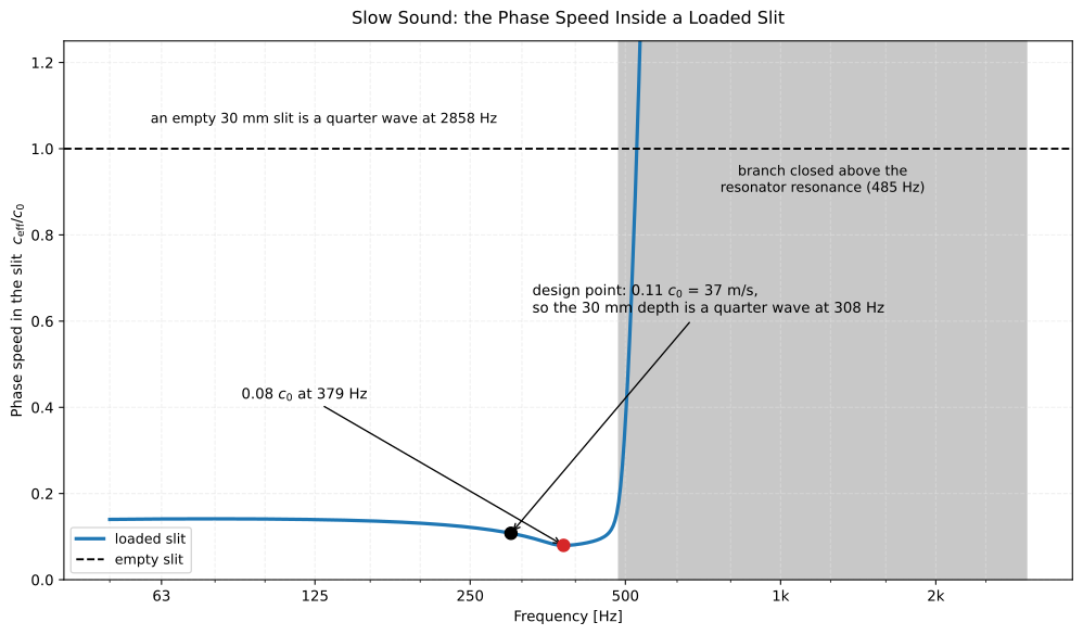
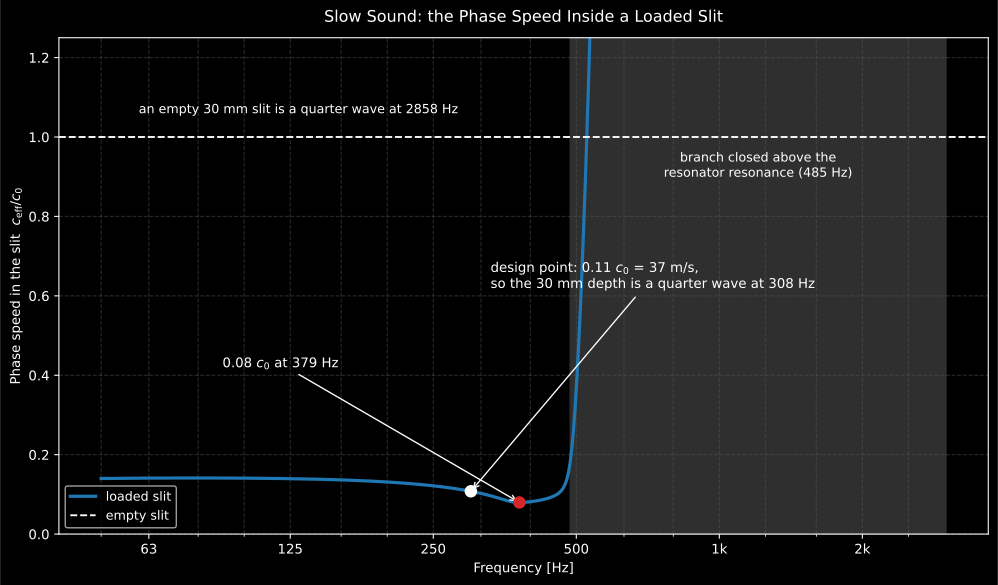
The mechanism the guide is named after, over frequency. The empty slit sits on 1 by definition; the loaded one falls to a minimum of 0.08 near 379 Hz and then climbs steeply as the resonators pass their own resonance at 485 Hz, above which the propagating branch closes. At the 300 Hz design point the phase speed is 0.11 = 37 m/s, which makes the fixed 30 mm depth a quarter wavelength at 308 Hz, where the panel resonates. The same 30 mm of plain air would be a quarter wave at 2858 Hz, and that ratio is the whole argument for the panel being thin. The same curve explains the 2 cm metadiffuser panel of the metadiffuser guide.
Show the code for this figure
f_sweep = np.geomspace(50.0, 3000.0, 400)swept = materials.slit_helmholtz_absorber( f_sweep, design.resonator, slit_height=design.slit_height, lattice_step=3.0e-2, period_m=5.0e-2,)c_ratio = 2 * np.pi * f_sweep / swept.effective_wavenumber.real / 343.0print(round(float(c_ratio.min()), 3), round(float(f_sweep[c_ratio.argmin()]))) # 0.08 381Where the effective wavenumber comes from
Section titled “Where the effective wavenumber comes from”The wavenumber the result returns is not a fitted number: it is the product of two visco-thermal models the library also exposes on their own. The empty slit already has a complex effective density and bulk modulus, set by the viscous and thermal boundary layers against its walls, which is why a sub-millimetre slit is lossy at all, and each resonator adds a shunt impedance in parallel with it.
# The empty slit, at the design frequency and slit height.rho_e, k_e = materials.slit_effective_properties(    np.array([300.0]), slit_height=design.slit_height)print(np.round(rho_e, 3))      # [1.355-0.203j]  against free air 1.205 kg/m^3print(f"{k_e[0]:.3e}")         # 1.332e+05+7.725e+03j  against adiabatic 1.419e+05 Pa
# One resonator's shunt impedance, either side of its own resonance at 484 Hz.z_hr = materials.helmholtz_resonator_impedance(    np.array([300.0, 484.0, 800.0]), design.resonator,    slit_height=design.slit_height, lattice_step=3.0e-2,)print(np.sign(z_hr.imag))      # [-1. -1.  1.]  compliance below, mass above
Below its own resonance the shunt is a compliance: it softens the slit
without adding moving mass, and that is exactly what lowers the phase speed.
materials.rectangular_duct_properties(f, side=1.0e-3) gives the same
effective pair for a square duct when the guiding geometry is a duct rather
than a slit, and all three take an AirProperties state (speed of sound,
density, viscosity, Prandtl number, heat-capacity ratio, atmospheric
pressure), so a design for a hot exhaust duct or a cabin at altitude changes
one argument rather than the model.
4. Classical resonant absorbers through the same lens
Section titled “4. Classical resonant absorbers through the same lens”Critical coupling is not exclusive to metamaterials; it is the organising principle hiding inside the classical resonant absorbers of the porous and multilayer guide:
- The microperforated panel is a critically coupled absorber avant la lettre. Maa’s peak absorption equals one exactly when the normalised resistance , which is the impedance-matching condition of section 1 stated for a locally reacting sheet. An MPP over a cavity tuned to is doing precisely what the slit panel does, with the viscous loss provided by submillimetre holes instead of a submillimetre slit; what it cannot do is slow the sound. Its peak is the mass-spring resonance of the hole mass against the cavity compliance; conventional designs land the cavity around a tenth to a twentieth of a wavelength, so without the slow-sound compression the construction stops severalfold short of the loaded slit’s depth.
- Membrane and decorated-membrane absorbers trade the hole viscosity for the flexural loss of a limp sheet; the same loss-versus-leakage balance governs their peak, and adding masses to the membrane (the decorated membrane of the metamaterials literature) tunes the resonance downward the way the loading resonators tune the slit.
- The design question is always the same. Pick the resonance with the
geometry, then match the loss to the leakage. The porous-layer models ask
“how thick”; the resonant family asks “how lossy”, and
critical_coupling_designanswers it for the slit panel exactly.
The price of resonance is bandwidth, and it is worth a number rather than an adjective. The 300 Hz design keeps from 282 Hz to 320 Hz and from 266 Hz to 341 Hz, a third of an octave, against a 50 mm porous blanket that gives about 0.68 at 500 Hz and keeps working over decades above it. A metamaterial absorber is therefore a tool for a known tonal or modal problem, not a general treatment: it buys depth with bandwidth.
The usual answer is to stop asking one cell to do the work. Chaining resonators along one slit is what the library’s own list argument is for:
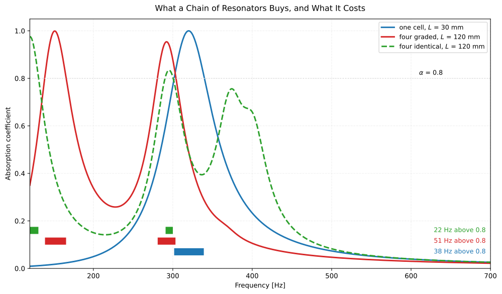
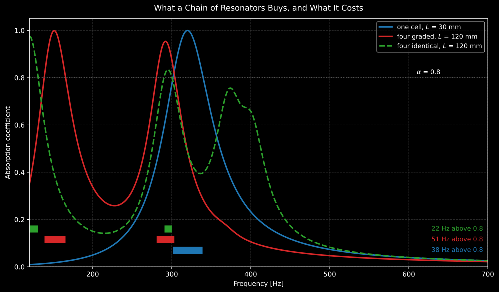
What a chain buys, and what it costs. Measured as the total frequency interval above , not as the span between the outermost points, which for a chain hides a dip: one cell gives 38 Hz, the four graded resonators give 51 Hz in two lobes, and four identical resonators of the same total depth give only 22 Hz. So the extra stages alone do not buy bandwidth: detuning them is what makes the depth pay, which is the whole idea behind the rainbow-trapping designs of Jiménez et al. (2017). The cost is geometric and unavoidable, since : the four-stage panel is 120 mm deep against the single cell’s 30 mm, and its slit height (1.2 mm here) is a compromise no longer critically coupled to any one stage.
Show the code for this figure
# `slit_helmholtz_absorber` takes a list: that is the chain along the slit.f_chain = np.linspace(120.0, 700.0, 700)graded = [materials.critical_coupling_design(target, base, lattice_step=3.0e-2, period_m=5.0e-2).resonator for target in (250.0, 320.0, 410.0, 520.0)]chain = materials.slit_helmholtz_absorber(f_chain, graded, slit_height=1.20e-3, lattice_step=3.0e-2, period_m=5.0e-2)step = float(f_chain[1] - f_chain[0])print(round(float(chain.absorption.max()), 3), round(float(np.sum(chain.absorption >= 0.8)) * step)) # 0.999 515. From the solver to a measured panel
Section titled “5. From the solver to a measured panel”Nothing above has been built. Four things stand between the solved geometry and a panel that can be put in front of an instrument.
The slit tolerance is a design parameter. The solved slit is 0.978 mm, and the loss balance is set by that sub-millimetre dimension. Holding the design frequency at 300 Hz, a slit machined 0.02 mm narrow or wide still gives ; at ±0.05 mm it is 0.982 and 0.984; at ±0.10 mm it has fallen to 0.931 and 0.939. So a few hundredths of a millimetre is the working tolerance, and a tenth is where the panel stops being perfect. Note which way the two errors fail: a narrow slit over-damps ( at −0.05 mm) and a wide one under-damps ( at +0.05 mm). Err wide. The visco-thermal model assumes smooth rigid walls, so additive-manufacturing roughness is extra loss that pushes an as-designed panel towards over-damping; a prototype cut slightly wide and trimmed converges from the right side.
A periodic panel does not fit an arbitrary tube. ISO 10534-2 Clause 6
requires a specimen with a regular lateral structure to be cut along the lines
of symmetry of that structure, and where the structural units do not fit the
tube cross-section, to be measured on several specimens with the cut moved
relative to the structure. The 50 mm period here does not fit a 29 mm tube at
all and fits a 100 mm circular tube only as two whole periods across one
diameter, which is not a symmetric cut. The clean route is a square or
rectangular tube whose side is an integer number of periods, with the rigid
tube walls acting as the symmetry planes of the infinite array, and then the
plane-wave ceiling has to be recomputed for that geometry with
plane_wave_frequency_range(..., shape="rectangular") on the maximum side
length, not on a nominal diameter.
Put the reference plane where the model does. The tube’s is the panel face, not the mouth of the slit and not the front of the frame; a millimetre of error there rotates the measured impedance without touching the absorption, exactly as the impedance-tube guide describes.
Or measure it as a surface. If the panel is meant for a room rather than for a duct, the honest verification is a 10–12 m² specimen in a reverberation room to ISO 354, and the result will be the random-incidence coefficient, not the the normal-incidence design promises, for the reason set out under off-normal incidence above.
What this guide covers
Section titled “What this guide covers”Covered
The slit + Helmholtz-resonator metamaterial absorber of Jiménez et al. (2016/2017): the transfer-matrix chain with the Stinson (1991) visco-thermal effective parameters, the resonator impedance with its radiation end corrections and the slit-radiation term (
slit_helmholtz_absorber, withHelmholtzResonatoras the geometry container and the retrievedeffective_wavenumberandeffective_impedanceexposed on the result), and the critical-coupling design solver (critical_coupling_design) that tunes cavity length and slit height until the reflection zero sits on the real-frequency axis. The two visco-thermal building blocks the chain is assembled from are exposed as well (slit_effective_properties,rectangular_duct_propertiesandhelmholtz_resonator_impedance, all taking anAirPropertiesstate), andslit_helmholtz_absorberaccepts a list of resonators, which is the graded chain of section 4.Not covered
No measurement standard governs these prediction models; section 5 sets out the route a built panel would be verified along, in the impedance tube (ISO 10534-2) or the reverberation room (ISO 354), but nothing here performs any of it: the tolerance and angle figures quoted are model evaluations, and the roughness of a printed slit, the frame, the mounting and the finite panel size are all outside the model. The membrane and decorated-membrane absorbers of section 4 are discussed as context only; the classical perforated, microperforated and membrane layers are implemented in Porous and Multilayer Absorbers, and the resonator-loaded slit used as a phase element rather than an absorber is the subject of Metadiffusers.
References
Section titled “References”- Cox, T. J., & D'Antonio, P. (2017). Acoustic absorbers and diffusers: Theory, design and application (3rd ed.). CRC Press. https://doi.org/10.1201/9781315369211ISBN 978-1-4987-4099-9. The classical resonant-absorber designs the metamaterial family extends.
- Jiménez, N., Groby, J.-P., Pagneux, V., & Romero-García, V. (2017). Iridescent perfect absorption in critically-coupled acoustic metamaterials using the transfer matrix method. Applied Sciences, 7(6), 618. https://doi.org/10.3390/app7060618The slit + Helmholtz-resonator transfer-matrix model and the critical-coupling (perfect-absorption) condition implemented in slit_helmholtz_absorber, plus the graded (iridescent) broadband chains of section 4.
- Jiménez, N., Huang, W., Romero-García, V., Pagneux, V., & Groby, J.-P. (2016). Ultra-thin metamaterial for perfect and quasi-omnidirectional sound absorption. Applied Physics Letters, 109(12), 121902. https://doi.org/10.1063/1.4962328The resonator impedance (Eq. A23), its radiation end corrections (Eqs. A24-A27), the worked slow-sound examples and the published lambda/88 perfect absorber cited in the introduction.
- Jiménez, N., Umnova, O., & Groby, J.-P. (Eds.). (2021). Acoustic waves in periodic structures, metamaterials, and porous media. Springer. https://doi.org/10.1007/978-3-030-84300-7Topics in Applied Physics, Vol. 143. The book-length treatment of critical coupling, slow sound and resonant metamaterial absorbers.
- Maa, D.-Y. (1998). Potential of microperforated panel absorber. The Journal of the Acoustical Society of America, 104(5), 2861-2866. https://doi.org/10.1121/1.423870The MPP impedance and design formulas whose r = 1 peak condition section 4 identifies with critical coupling.
- Stinson, M. R. (1991). The propagation of plane sound waves in narrow and wide circular tubes, and generalization to uniform tubes of arbitrary cross-sectional shape. The Journal of the Acoustical Society of America, 89(2), 550-558. https://doi.org/10.1121/1.400379The visco-thermal effective density and bulk modulus of the slit and of the square necks and cavities.