In-situ Road-Surface Absorption

How much sound a road surface absorbs decides how loud its traffic is, and a core cannot be cut out of a motorway and carried to a laboratory. ISO 13472 measures the absorption in situ, on the pavement as built, twice over. The subtraction technique of Part 1 fires an impulse from a loudspeaker down onto an extended surface and separates the incident and reflected components of one microphone’s impulse response in time; the spot method of Part 2 seals a short tube onto a small patch and hands the mathematics to the impedance-tube transfer-function method. This guide covers both, from the mandatory geometry and the Adrienne window to the sampled area and the plane-wave limits of the tube, and closes with the choice between them.

1. Subtraction technique (ISO 13472-1)

Out in the field there is no reverberation room. ISO 13472-1 measures the sound absorption of a road surface (or any extended flat surface) in situ by firing an impulse from a loudspeaker at height $d_{s}$ down onto the surface and recording the impulse response at a microphone at height $d_{m}$ . The incident and reflected components are separated in time with an Adrienne window; their transfer function gives the reflection factor and hence the absorption.

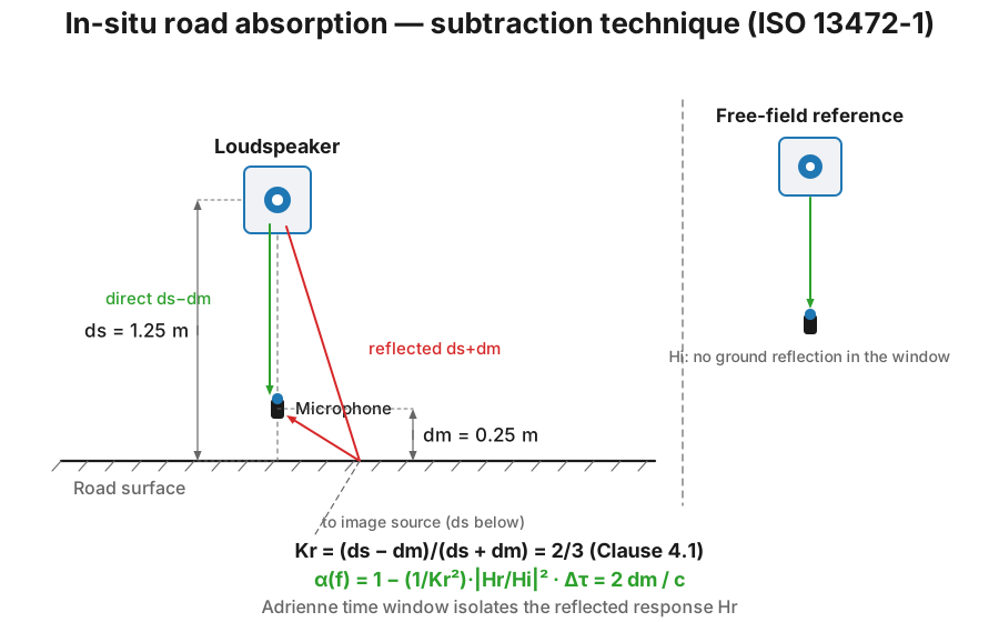
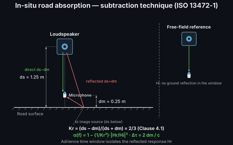
ISO 13472-1 in-situ road absorption by the subtraction technique: a loudspeaker at 1.25 m and a microphone at 0.25 m above the road surface, with the direct and road-reflected ray paths and a free-field reference measurement, the reflected component isolated by an Adrienne time window

Geometrical spreading (Clause 4.1). The reflected wave travels farther than the direct wave, so it is attenuated by the geometrical-spreading factor

K_{r} = \frac{d _{s} - d _{m}}{d _{s} + d _{m}},

which equals $2/3$ for the mandatory geometry $d_{s} = 1.25$ m, $d_{m} = 0.25$ m. Both heights are held to within 0.005 m through the averaging, and the acoustic centres of source and microphone lie on one line normal to the surface with the microphone axis parallel to it. The absorption follows from the windowed incident and reflected spectra $H_{i}$ , $H_{r}$ :

α (f) = 1 - \frac{1}{K _{r}^{2}} \frac{H _{r} ( f )}{H _{i} ( f )}^{2} .

1.1 What is subtracted

The microphone hears the direct wave and the road reflection in the same impulse response, and the mandatory geometry puts them only $2 d_{m} / c \approx 1.5$ ms apart — far too little to gate apart at the bottom of the reported band. ISO 13472-1 therefore requires the subtraction technique (Clause 4.2) rather than plain time windowing, and that is the step the two arrays this page’s functions consume come out of:

Rig the source and the microphone so that their separation cannot change: the standard asks for a fixed, stable mechanical connection between them, because the subtraction is a cancellation of two nominally identical waveforms.
Measure over the road and average until the impulse response is stable — at least 50 responses (Clause 4.3), which is what beats the background noise and the meteorological variation.
Repeat the identical measurement with the rig taken away from any reflecting surface. That free-field response is $h_{i}$ . Correct any residual time shift between the two takes, and make them within a short time of each other — the standard recommends under 10 minutes — because the delay is temperature dependent.
Subtract: $h_{r} = h_{road} - h_{i}$ . Everything the two takes share — the direct wave, the loudspeaker, the microphone, the whole chain — cancels, and what survives is the surface reflection alone.
Window $h_{i}$ and $h_{r}$ with the same window applied at their own arrival times ( $T_{w, direct} = T_{w, reflected}$ ), transform, and form $α$ with $K_{r}$ .

Two acceptance conditions ride on that chain. The signal-to-noise ratio must exceed 10 dB in every one-third-octave band from 250 Hz to 4 kHz (Clause 7.4), and no calibration of level is needed at all — the method is a ratio of two transfer functions from the same chain (Clause 6.1) — but the Annex B reference measurement of section 1.2 is not optional for the same reason. The snippets below start from an hi and an hr that stand in for that pair; in the field they are the free-field reference and the windowed road reflection, in that order.

import numpy as np
from phonometry import materials

# A band-limited incident impulse response and a synthetic road reflection
# hr = Kr * r0 * delayed(hi): a reflection of magnitude r0 = 0.4, delayed by the
# extra path, and scaled by the geometrical-spreading factor Kr.
fs, n = 48000.0, 4096
t = np.arange(n) / fs
hi = np.zeros(n)
hi[:64] = np.hanning(64) * np.cos(2.0 * np.pi * 1500.0 * t[:64])

kr = materials.geometric_spreading_factor()          # (ds - dm)/(ds + dm) = 2/3
hr = kr * 0.4 * np.roll(hi, 96)

# Narrow-band absorption, then reduced to one-third octaves over 250-4000 Hz.
alpha = materials.insitu_absorption_coefficient(hi, hr)   # 1 - (1/Kr^2)|Hr/Hi|^2
freq = np.fft.rfftfreq(n, 1.0 / fs)
centres, band = materials.one_third_octave_absorption(freq, alpha)
print(round(kr, 4))                # 0.6667
print(round(float(band[2]), 3))    # 0.84  (alpha = 1 - 0.4^2 = 0.84)

1.2 The reference surface (Annex B)

The raw ratio $∣ H_{r} / H_{i} ∣^{2} / K_{r}^{2}$ assumes that the electro-acoustic chain and the geometry factor cancel exactly. They do not: the loudspeaker and the microphone have their own responses along paths of different length, and the mandatory $K_{r} = 2/3$ is a plane-wave idealisation of a finite geometry. At the bottom of the band, where a dense road absorbs a few percent, that residual error is comparable with the quantity being measured — which is why Annex B makes a reference measurement mandatory, not advisory.

The fix is one extra measurement per set-up. Lay a highly reflecting plate — plane, smooth, dense and jointless, and large enough to cover the whole maximum sampled area — on the same spot, and repeat the entire procedure over it with the rig geometry unchanged. The measured pressure reflection factor of the reference is then the chain’s own error function $e (f)$ , because the plate itself reflects everything; dividing the road’s measured factor by it removes $e (f)$ and, since the geometry is identical, the $K_{r}$ factor with it:

α_{road} (f) = 1 - \frac{Q _{p, road,meas} ( f )}{Q _{p, ref,meas} ( f )}^{2} .

import numpy as np

# `materials` is imported by the block above. Two complex pressure reflection
# factors from the identical set-up: one over the road, one over the reference
# plate. Their ratio is Annex B.
freq = np.array([250.0, 500.0, 1000.0, 2000.0, 4000.0])
q_road = np.array([0.97, 0.94, 0.88, 0.72, 0.55]) * np.exp(-0.05j * freq / 1e3)
q_ref = np.array([1.02, 1.01, 1.00, 0.99, 0.98]) * np.exp(-0.05j * freq / 1e3)
print(np.round(materials.absorption_reference_corrected(q_road, q_ref), 3))
# [0.096 0.134 0.226 0.471 0.685]

# Uncorrected, the same road data would read:
print(np.round(1.0 - np.abs(q_road) ** 2, 3))
# [0.059 0.116 0.226 0.482 0.698]

The plate must itself be verified: a sample of its material is measured in an impedance tube per ISO 10534-1 or ISO 10534-2 to confirm an absorption coefficient below 0.05 over the reported range, which is what licenses the assumption $∣ Q_{p, ref} ∣ = 1$ . A portable reference surface must also be rigid enough that it cannot resonate. In practice the reference is the first thing to reach for when a measured spectrum shows small negative absorptions in the lowest bands: as the printed values above show, the correction moves the 250 Hz band by more than the value itself.

Adrienne window (Clause 6.4). The time window that isolates the reflection mandates only a sharp leading edge, a 5 ms flat portion and a cosine-squared or Blackman-Harris trailing edge; the exact durations are reported per measurement, not fixed, so they are configurable here.

from phonometry import materials

# Default: 0.5 ms leading edge, 5 ms flat top, 5 ms Blackman-Harris trailing.
w = materials.adrienne_window(48000.0)
print(w.shape[0])          # 504 samples at 48 kHz
print(round(float(w.max()), 3))   # 1.0  (flat top and edges meet at unity)

That length is the method’s single free parameter, and it is a trade with two ends. The total window duration sets the lowest frequency the transform can resolve — 10.5 ms is about 95 Hz, and a 220 Hz lower limit needs roughly 5 ms of flat portion, which is why the reported band starts at 250 Hz and not lower. Lengthening it buys low-frequency validity, and every millisecond added also admits reflections from the mast, the vehicle, the operator and anything else within the corresponding radius, and enlarges the patch of road that contributes to the answer. The practical rule: choose the longest window that stays clear of the first parasitic arrival visible in the raw impulse response, apply the same window to the free-field reference and to the reflection, and report the shape and the durations with the result, since the standard fixes neither and two laboratories using different windows are not measuring the same thing. A spectrum that rises implausibly in the lowest reported bands is the usual sign of a window that is too short, or of a parasitic arrival inside it.

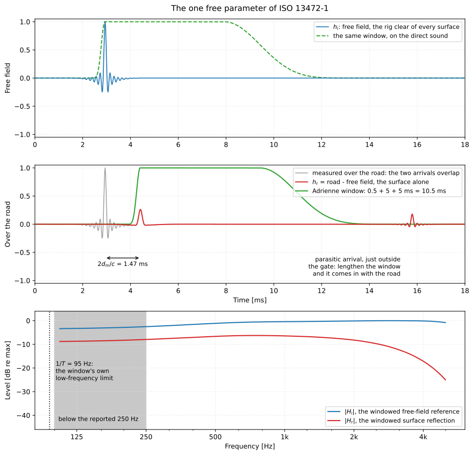
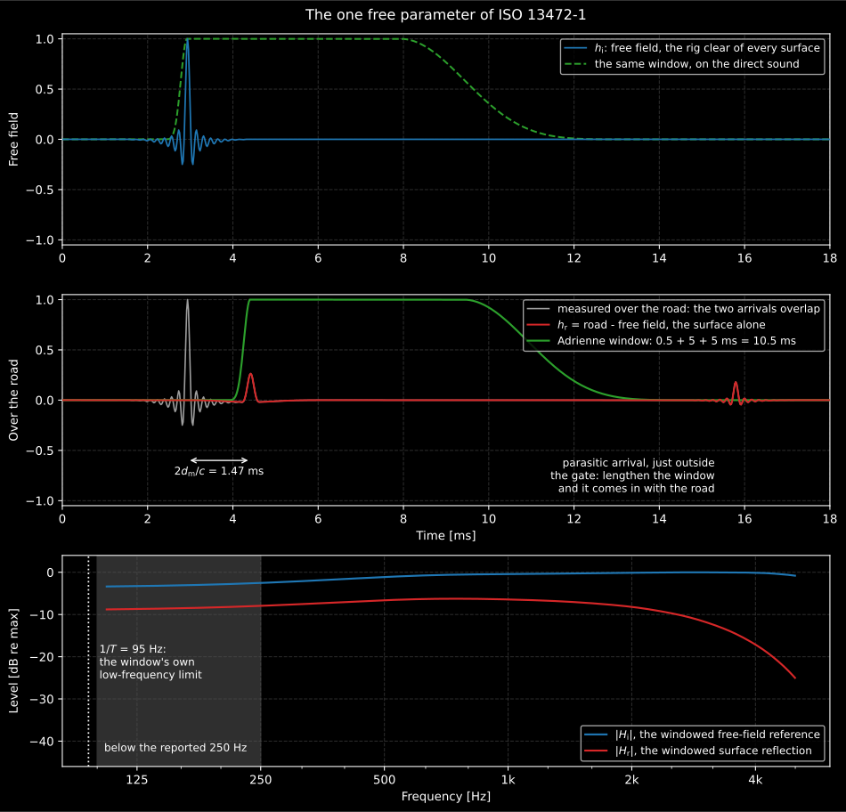
Three stacked panels on a common time axis: the free-field reference impulse response with the Adrienne window placed on the direct sound; the response measured over the road where the direct and reflected arrivals overlap, their 1.47 millisecond separation dimensioned, the subtracted surface reflection and the 10.5 millisecond Adrienne window drawn over it with a parasitic arrival just outside the gate; and the resulting windowed incident and reflected spectra with the 95 hertz reciprocal-window limit marked and the region below the reported 250 hertz band shaded

The whole method in three traces. The two arrivals are 1.47 ms apart on the mandatory geometry, so no gate separates them; the middle panel’s red trace is what subtraction leaves once the free-field reference has been taken away. The green gate is the Adrienne window at its default 0.5 + 5 + 5 ms, whose total duration sets both the 95 Hz floor marked in the bottom panel and the 1.34 m radius of road that contributes. The parasitic arrival at 15.8 ms is outside it — and would not be if the window were lengthened to reach lower in frequency.

Show the code for this figure

import matplotlib.pyplot as plt
import numpy as np

# `materials` is imported above. The window itself, placed at the reflected
# arrival of the mandatory geometry (2 dm / c after the direct sound).
fs = 48000.0
w = materials.adrienne_window(fs)
t = np.arange(w.size) / fs + (1.5 / 340.0) - 0.5e-3
fig, ax = plt.subplots()
ax.plot(t * 1e3, w)
ax.axvline(1.0 / 340.0 * 1e3, linestyle=":", label="direct arrival")
ax.axvline(1.5 / 340.0 * 1e3, linestyle="--", label="reflected arrival")
ax.set_xlabel("Time [ms]")
ax.set_ylabel("Window")
ax.legend()
plt.show()

End-to-end spectrum. insitu_absorption_spectrum runs the whole chain (the windowed incident and reflected impulse responses to the narrow-band absorption and on to one-third-octave bands) and returns a plottable InsituAbsorptionResult:

import numpy as np
from phonometry import materials
from scipy.signal import firwin, lfilter

# A synthetic-but-realistic measurement. hi is a unit incident impulse; the road
# reflection hr = Kr * r0 * roll(hi, shift) uses the geometrical-spreading
# factor Kr, a mildly frequency-dependent r0 (a gentle low-pass, so a porous
# surface reflects less as frequency rises) and the reflected-path delay
# shift = round(2 dm / c * fs).
fs, n = 48000.0, 8192
kr = materials.geometric_spreading_factor()           # (ds - dm)/(ds + dm) = 2/3
hi = np.zeros(n)
hi[0] = 1.0
taps = firwin(41, 1200.0, fs=fs)
taps = taps / taps.sum()
shift = int(round(2.0 * 0.25 / 340.0 * fs))     # reflected-path delay 2 dm / c
hr = kr * 0.85 * np.roll(lfilter(taps, 1.0, hi), shift)

result = materials.insitu_absorption_spectrum(hi, hr, fs)
print(result.frequencies[[0, -1]].astype(int))     # [ 250 4000]
print(np.round(result.absorption[[0, 6, 12]], 2))  # [0.31 0.65 1.  ]
result.plot()   # alpha(f) bar chart over 250-4000 Hz (needs matplotlib)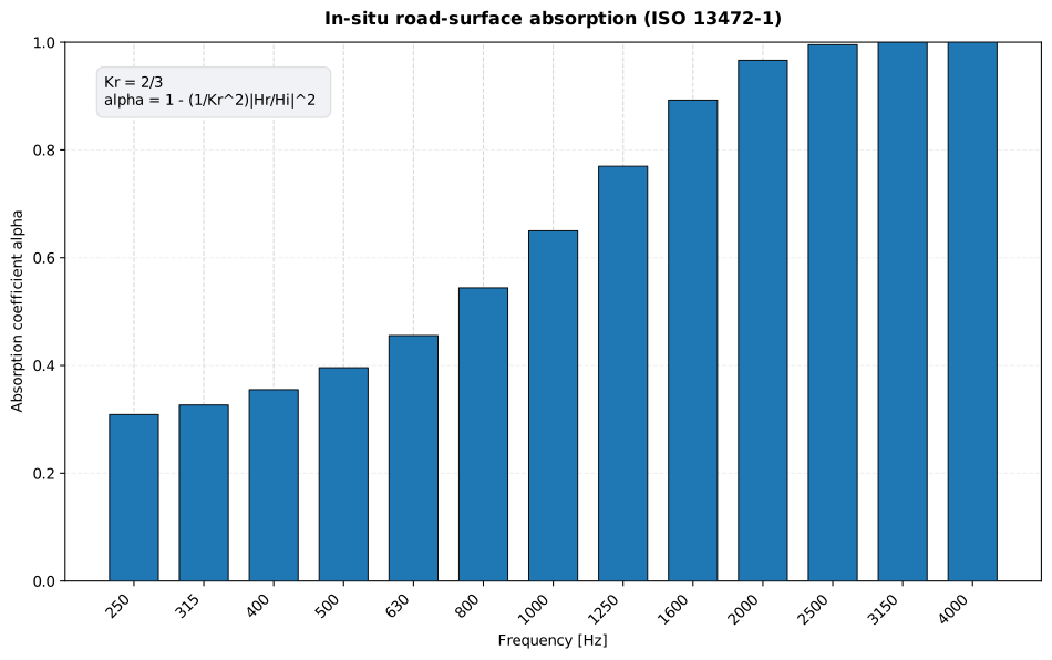

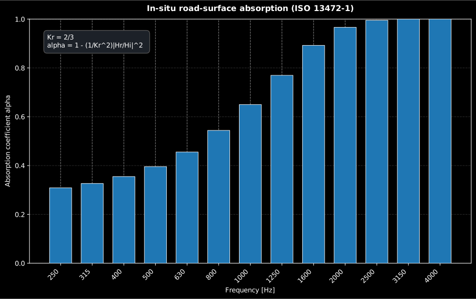
An in-situ one-third-octave road-surface absorption spectrum computed by the reflection-factor route from a synthetic road reflection, rising from about 0.3 at 250 Hz to near 1.0 above 2 kHz

The absorption rises with frequency because the surface reflects less of the high-frequency energy, exactly as the low-pass reflection factor $r_{0} (f)$ dictates through $α = 1 - (1/ K_{r}^{2}) ∣ H_{r} / H_{i} ∣^{2}$ .

Show the code for this figure

import matplotlib.pyplot as plt
import numpy as np
from scipy.signal import firwin, lfilter
from phonometry import materials

# A synthetic-but-realistic measurement. hi is a unit incident impulse; the road
# reflection hr = Kr * r0 * roll(hi, shift) uses the geometrical-spreading
# factor Kr, a mildly frequency-dependent r0 (a gentle low-pass, so a porous
# surface reflects less as frequency rises) and the reflected-path delay
# shift = round(2 dm / c * fs).
fs, n = 48000.0, 8192
kr = materials.geometric_spreading_factor()           # (ds - dm)/(ds + dm) = 2/3
hi = np.zeros(n)
hi[0] = 1.0
taps = firwin(41, 1200.0, fs=fs)
taps = taps / taps.sum()
shift = int(round(2.0 * 0.25 / 340.0 * fs))     # reflected-path delay 2 dm / c
hr = kr * 0.85 * np.roll(lfilter(taps, 1.0, hi), shift)
result = materials.insitu_absorption_spectrum(hi, hr, fs)

# result is the InsituAbsorptionResult computed above. One line:
result.plot()
plt.show()

# By hand: a bar chart of alpha over the one-third-octave bands.
freqs = result.frequencies
positions = np.arange(freqs.size)
fig, ax = plt.subplots()
ax.bar(positions, np.nan_to_num(result.absorption), width=0.7, color="#1f77b4")
ax.set_xticks(positions)
ax.set_xticklabels([f"{f:g}" for f in freqs], rotation=45, ha="right")
ax.set_xlabel("Frequency [Hz]")
ax.set_ylabel("Absorption coefficient alpha")
ax.set_ylim(0.0, 1.0)
ax.set_title("In-situ road-surface absorption (ISO 13472-1)")
plt.show()

Maximum sampled area (Annex A). The finite time window limits how much of the surface contributes to the reflection. The maximum sampled area is a circle whose radius the library computes from the geometry and window width; the Annex A worked example ( $d_{s} = 1.25$ m, $d_{m} = 0.25$ m, $c = 340$ m/s, 5 ms flat window) gives about 1.34 m.

from phonometry import materials
print(round(materials.max_sampled_area_radius(5.0e-3), 3))   # 1.343  (metres)

The whole arrangement fits in one to-scale drawing. plot_insitu_geometry draws the standard set-up with that sampled radius on the surface, and a measured InsituAbsorptionResult that retained its heights redraws its own with result.plot_geometry().

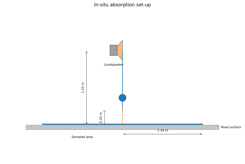
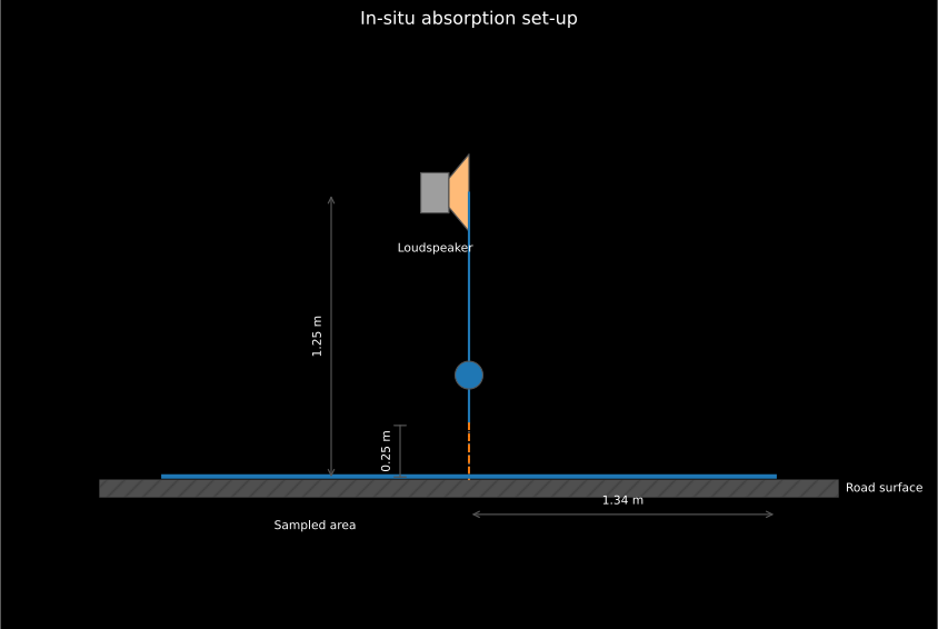
To-scale side view of the in-situ absorption set-up: the loudspeaker on its mast 1.25 m above the hatched road surface, the microphone on the same vertical at 0.25 m, the dashed surface-reflected path below it and the 1.34 m radius of the sampled area dimensioned on the surface

The standard geometry to scale: source at 1.25 m, microphone at 0.25 m on the same vertical, and the 5 ms window turned into the 1.34 m radius of road that actually contributes to the reflection.

Show the code for this figure

import matplotlib.pyplot as plt
from phonometry import materials

# The standard geometry: source at 1.25 m, microphone at 0.25 m, and the
# 1.34 m sampled-area radius of the 5 ms window.
materials.plot_insitu_geometry()
plt.show()

# A measured spectrum retains its heights and redraws its own set-up:
#   result = materials.insitu_absorption_spectrum(hi, hr, fs)
#   result.plot_geometry()

1.3 Before you press record

That radius is not a number to admire; it is a clearance you walk. Compute it, pace it out, and check what is inside. ISO 13472-1 Clauses 7 and 8 give the gates that decide whether a measurement may be made at all, and they, not the signal processing, are what usually invalidates a roadside campaign.

The maximum sampled area must be clear. Any object other than the pavement — a fence, a rock, a barrier, a parked car — is a reflecting object. None may be inside the sampled area, and anything outside it must be farther from the microphone than $d_{s}$ , that is farther than 1.25 m. The microphone stand itself must not influence the measurement.
The surface must be visually homogeneous and free of changes in the material, and it must be dry. On a surface with a significant void content, verify that the pores are dry too, not just the surface. Wet measurements are legitimate for research, and their results cannot be used to classify or qualify a surface.
Wind at microphone height must not exceed 5 m/s.
Temperature: ambient air between 0 °C and 35 °C, and the road surface between 0 °C and 50 °C.
The reference surface of section 1.2 must cover at least the same sampled area, so the radius sizes the plate you have to carry as well as the clearance you have to find.

The measurement itself is a thirteen-step procedure whose order matters: check the surface and the weather, place the rig, compute and walk the radius, choose the source and the signal, average at least 50 responses over the road, take the free-field reference with the rig clear of everything, subtract, window, transform, form the reflection factor with $K_{r}$ , repeat the whole thing over the reference plate, and only then average into one-third octaves. A result reported without the window shape and durations, and without the reference measurement, is not an ISO 13472-1 result.

1.4 When the site forces an angle

Everything above is the mandatory normal-incidence geometry: source and microphone on the same vertical over the surface. Annex F provides for an oblique arrangement, and the library follows it. Two things change and both are exposed:

The geometrical-spreading factor acquires an angular form, $K_{r, θ}^{2} = 1 - cos^{2} θ (1 - K_{r}^{2})$ , computed by geometric_spreading_factor_angle and used automatically when insitu_absorption_spectrum is given an incidence_angle. Both take the angle in radians, unlike the degrees the rest of this page quotes.
The sampled area stops being the circle in the figure above. It becomes the intersection of the surface with an ellipsoid of revolution whose foci are the source and the microphone, so it is an ellipse stretched along the direction of incidence, whose major axis msa_major_axis returns from the window width and the projected source-to-microphone distance. At 30° the 1.34 m circle becomes an ellipse 3.43 m along its major axis, so the clear zone to be checked grows with the angle and the measurement averages over more pavement, and less symmetrically.

import numpy as np

# `materials` is imported above. Thirty degrees off normal, with the same two
# heights: the spreading factor rises towards one and the sampled area stops
# being a 1.34 m circle. Both helpers take the angle in RADIANS.
print(round(float(materials.geometric_spreading_factor()), 4))           # 0.6667
print(round(float(materials.geometric_spreading_factor_angle(
    np.radians(30.0))), 4))                                              # 0.7638

# The projected source-to-microphone distance on the surface, (ds + dm) tan(theta),
# is what stretches the ellipse.
dp = 1.5 * np.tan(np.radians(30.0))
print(round(dp, 3))                                                      # 0.866
print(round(float(materials.max_sampled_area_radius(5.0e-3)), 3))        # 1.343
print(round(float(materials.msa_major_axis(5.0e-3, dp)), 3))             # 3.432

Keep the normal-incidence geometry wherever the site allows it: it is the arrangement the comparison with the spot method assumes, and the one published road data are quoted for.

2. Spot method (ISO 13472-2)

For smaller patches, ISO 13472-2 seals a short circular tube onto the surface and measures the absorption with the two-microphone transfer-function method of ISO 10534-2. The library provides the spot-method geometry and validity helpers; the transfer-function DSP itself is the impedance-tube routine two_microphone_impedance (see the Impedance Tube guide).

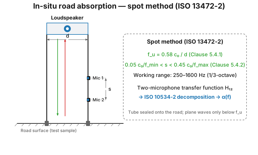
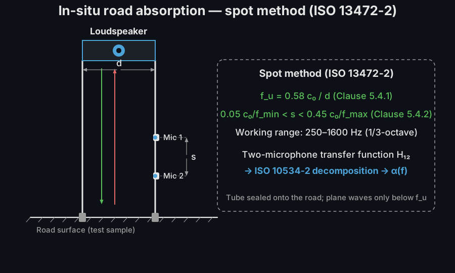
ISO 13472-2 spot method: a short circular tube sealed onto the road surface with a loudspeaker at the top and two microphones flush in the tube wall at spacing s, measuring absorption over 250 to 1600 Hz via the ISO 10534-2 two-microphone transfer-function method

The apparatus is a portable impedance tube stood on end: a loudspeaker at the top, two flush-mounted microphones at spacing $s$ in the tube wall, and the road surface itself as the sample. A test fixture with a ring of deformable material (a rubber O-ring or similar) makes an airtight seal between the tube mouth and the pavement, so the patch under the mouth, not the leak around it, terminates the tube; the underside of that sealing device defines the plane of reference at which the reflection factor is evaluated. The method is written for reflective surfaces, dense asphalts and test tracks per ISO 10844 rather than open porous layers: the standard declares it unreliable once the measured absorption coefficient exceeds 0.15, and no longer calls a surface reflective above 0.10, because on an absorbing surface the reflected wave the two microphones must resolve all but vanishes. The tube samples only the circle under its mouth, so one reading is a spot in the statistical sense too: on regular roads the standard spaces measurement positions over the area of interest with an emphasis on the wheel tracks (as a guideline, one position every 10 m), on a surface that must be smooth, flat, free of debris and dry.

Plane-wave limits (Clause 5.4). The tube supports only plane waves below

f_{u} = 0.58 \frac{c _{0}}{d},

with $d$ the tube diameter, and the microphone spacing $s$ must sit between $0.05 c_{0} / f_{min}$ and $0.45 c_{0} / f_{ma x}$ . The reported range is the one-third-octave bands 250–1600 Hz, and the standard’s own definition of a frequency range is by band edges: those centre frequencies mean 220 Hz to 1800 Hz in narrow bands, which is where the two arguments below come from.

from phonometry import materials

# Upper usable frequency of a 100 mm tube and the valid spacing window.
print(round(materials.spot_tube_upper_frequency(0.100, 343.0), 1))      # 1989.4 Hz
# 220 Hz and 1800 Hz are the outer edges of the 250 Hz and 1600 Hz bands.
s_min, s_max = materials.spot_microphone_spacing_bounds(
    343.0, f_min=220.0, f_max=1800.0)
print(round(s_min, 3), round(s_max, 3))    # 0.078 0.086  (metres)

Three numbers, three different limits, and they do reconcile. The 1989 Hz is the plane-wave ceiling of the 100 mm bore; the reported range stops one band below it because a band is only usable when its whole width is inside the valid range, and the 1600 Hz band reaches 1800 Hz. The 250 Hz floor is a spacing limit, not a length limit: below $f_{min}$ the two microphones are closer than 5 % of a wavelength apart and there is no phase difference left to resolve. Tube length answers a different question — it must be long enough for a plane wave to form, which Clause 5.4.2 meets by putting the microphones at least $3 d$ from the source (a minimum length of 480 mm for the 100 mm tube). The resulting spacing window, 78 mm to 86 mm here, is why the standard specifies $(81 \pm 4)$ mm for a single microphone pair. It is a narrower window than the 250–4000 Hz of the subtraction technique. Within it, the reduction is the ISO 10534-2 chain unchanged: the transfer function between the two microphones separates incident and reflected waves, and the standard’s Annex A additionally subtracts the internal losses of the system (measured once against a rigid plate) so the tube’s own dissipation is not billed to the road; that correction is spot_internal_loss_correction.

2.1 A position, step by step

The tube is portable and the procedure is short, which is exactly why it is worth writing down: almost everything that goes wrong with a spot measurement goes wrong in the two minutes before the source is switched on. Clauses 6 to 8 give the order.

Check the gates first. The surface must be smooth, flat, free of debris and dry; the air between 5 °C and 30 °C and the road surface between 5 °C and 45 °C, out of direct sunlight and away from strong heat sources — test at night where that cannot be met. If any of these fails, the measurement cannot be carried out.
Warm up. Switch the system on and leave it running for at least 15 minutes. The method lives on phase accuracy, and the electronics, the loudspeaker coil and the tube itself all have to be thermally stable.
Calibrate the microphones by the ISO 10534-2 Clause 7.5 procedure, before each measurement series and after each hour of measurement, for every microphone position used. That calibration is what corrects the phase and amplitude mismatch between the two capsules.
Take the reference measurement on a totally reflective specimen — a 10 mm steel plate is the standard’s own example. Its one-third-octave absorption must come out below 0.03; the result feeds the Annex A internal-loss correction, and it is taken at the same location immediately before or after the series.
Measure the background with the source off, and require at least 10 dB signal-to-noise in every band against it. Stay at least 25 m from passing heavy vehicles and motorcycles, and discard any run a passing vehicle disturbed.
Seal. Lay a bead of sealant in the fixture’s groove, sized to the surface texture — a few millimetres on a smooth surface, thicker on a coarse one. Press the fixture onto the road: the right amount is when a little material squeezes out. If almost none does, lift the fixture, check for a continuous circular impression, add sealant and repeat. Then mount the tube without moving the fixture and check for leaks around the perimeter, for instance by listening through an open tube.
Run and check. Average until the result is stable, or over 50 sweeps or bursts if there is no live read-out. If the signal-to-noise ratio is too low, raise the source level, remove the noise source or wait.
Verify the seal again. Lift the fixture and confirm the sealing material was in tight contact in a closed circle. If in doubt, re-seal and repeat the position — an air leak reads as absorption and there is nothing in the data to distinguish the two.

Two more things about the reduction. Systems commonly carry two microphone pairs and splice their narrow-band results, each pair over the part of the band where its spacing is optimal (spot_microphone_spacing_bounds gives that window for any pair). And the Annex A internal-loss correction is applied after the narrow-band results have been averaged into one-third octaves and before negative bands are clipped to zero — the standard deliberately lets the FFT produce negative narrow-band values and clips only at the end. Finish by repeating at at least four positions and reporting the mean and the standard deviation per band.

Subtraction or spot?

The two parts of ISO 13472 are complements, not competitors, and Part 2’s own introduction says both should give similar results between 315 Hz and 1600 Hz while their fields of application differ:

Surface type. The subtraction technique handles the full range from reflective to highly absorbing (porous asphalt included); the spot method is scoped to reflective surfaces and declared unreliable above a measured absorption of 0.15, where its confined reflected wave is no longer strong enough to resolve.
Sampled area. The subtraction technique averages over a patch whose Annex A clear zone extends to the 1.34 m maximum sampled-area radius of section 1 (about 5.6 m² of pavement, with the area actually contributing at each frequency set by the time window), a fair sample of texture and joints; the spot method sees only the patch under the tube mouth, so it trades spatial representativeness for the ability to sit on a narrow strip, a wheel track, or a laboratory core.
Bandwidth. 250–4000 Hz against 250–1600 Hz, which matters because the tyre-road noise the measurement usually serves peaks around 1 kHz but has content beyond the spot method’s ceiling.
Logistics. The subtraction rig needs a mast, a free-field reference measurement and a pause in traffic; the spot tube needs a flat, sealable patch and minutes per point. Surface types and acceptance criteria aside, that practical difference is usually what decides.

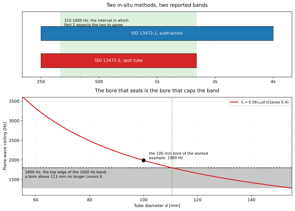
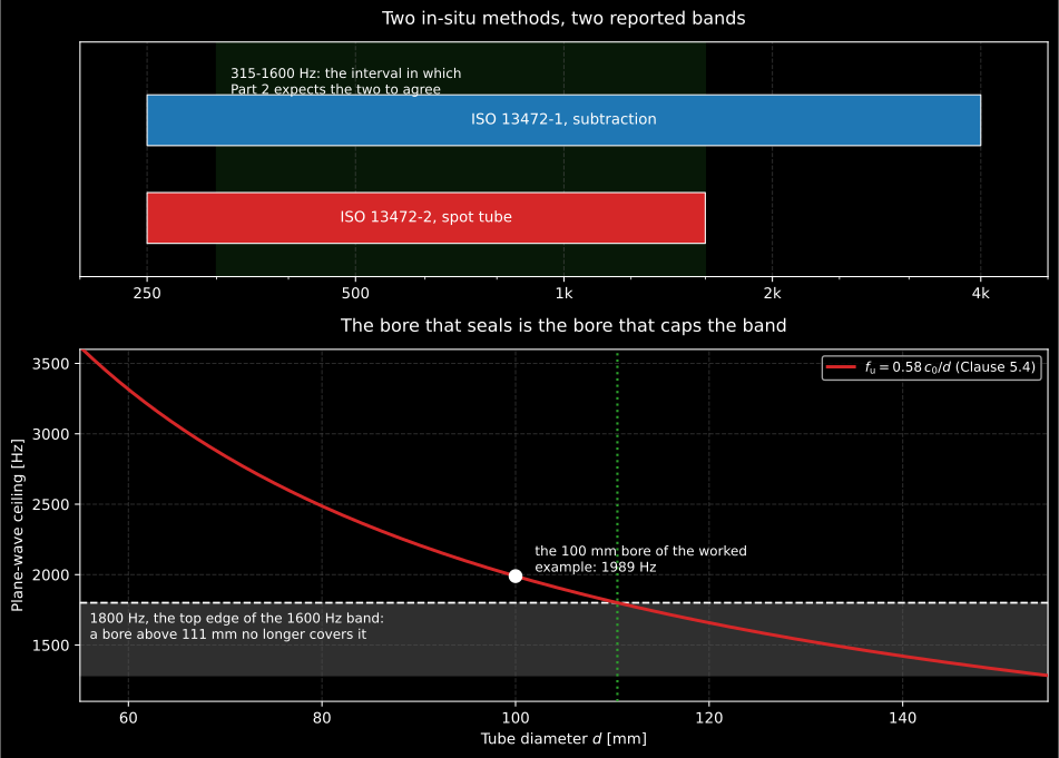
Two panels: on top, the reported one-third-octave ranges of the two methods drawn as bars on a common log-frequency axis, 250 to 4000 hertz for the subtraction technique and 250 to 1600 hertz for the spot tube, with the 315 to 1600 hertz interval where Part 2 expects them to agree shaded; below, the plane-wave ceiling of the spot tube falling as the bore grows, the 100 millimetre worked example marked at 1989 hertz and the region below the 1800 hertz top band edge shaded to show that a bore above 111 millimetres no longer covers the reported range

Why the choice is made on bandwidth as much as on logistics. The spot tube’s ceiling is set by its own bore, and the bore has two jobs that pull against each other: it must be wide enough to seal on a textured pavement and narrow enough to keep plane waves up to the top of the reported range. At 111 mm the two requirements meet; beyond it the 1600 Hz band is no longer covered. The shaded interval on top is where Part 2’s introduction expects the two methods to agree, and it is also the interval a comparison between them should be judged on.

Show the code for this figure

import matplotlib.pyplot as plt
import numpy as np

# `materials` is imported above. The plane-wave ceiling against the bore.
bores = np.linspace(0.055, 0.155, 300)
ceiling = [materials.spot_tube_upper_frequency(d, 343.0) for d in bores]
fig, ax = plt.subplots()
ax.plot(bores * 1e3, ceiling)
ax.axhline(1800.0, linestyle="--")     # top edge of the 1600 Hz band
ax.set_xlabel("Tube diameter d [mm]")
ax.set_ylabel("Plane-wave ceiling [Hz]")
plt.show()

Both methods report the same quantity, the normal-incidence absorption coefficient in one-third-octave bands, so a low-absorption lane can be surveyed with the spot tube and anchored with a subtraction measurement at a few positions.

What this guide covers

Covered
ISO 13472-1:2002’s subtraction technique: the Clause 4.1 geometrical spreading (materials.geometric_spreading_factor), the Clause 6.4 Adrienne time window (materials.adrienne_window), the narrow-band and one-third-octave reduction (materials.insitu_absorption_coefficient, materials.one_third_octave_absorption, materials.insitu_absorption_spectrum) and the Annex A sampled-area radius (materials.max_sampled_area_radius), with the Annex B reference-surface correction (materials.absorption_reference_corrected) and the Annex F oblique-incidence case (materials.geometric_spreading_factor_angle, materials.msa_major_axis, and the incidence_angle argument of materials.insitu_absorption_spectrum); and ISO 13472-2:2010’s spot-method plane-wave frequency limit, microphone-spacing geometry and Annex A internal-loss correction (materials.spot_tube_upper_frequency, materials.spot_microphone_spacing_bounds, materials.spot_internal_loss_correction).
Not covered
Both in-situ road standards have since been revised (ISO 13472-1:2022, ISO 13472-2:2025); only the earlier 2002 and 2010 editions are implemented here, as the reference notes above flag. ISO 13472-2’s own transfer-function processing is not implemented in this module either: only the geometry, validity and correction helpers are provided, and the actual two-microphone DSP is the ISO 10534-2 routine of the Impedance Tube guide. Neither the acquisition itself nor the field gates are enforced anywhere in code: the averaging, the free-field reference, the signal-to-noise checks, the seal verification and the weather limits of sections 1.1 to 1.4 and 2.1 are the operator’s, and the library only sees the two arrays that come out of them.

References

International Organization for Standardization. (1998). Acoustics — Determination of sound absorption coefficient and impedance in impedance tubes — Part 2: Transfer-function method (ISO 10534-2:1998). The two-microphone transfer-function reduction the spot method reuses, implemented in the Impedance Tube guide.
International Organization for Standardization. (2002). Acoustics — Measurement of sound absorption properties of road surfaces in situ — Part 1: Extended surface method (ISO 13472-1:2002). The subtraction technique of section 1: the mandatory geometry, the Adrienne window and the Annex A sampled-area radius. Since revised as ISO 13472-1:2022 (https://www.iso.org/standard/77032.html); the 2002 edition is the implemented one.
International Organization for Standardization. (2010). Acoustics — Measurement of sound absorption properties of road surfaces in situ — Part 2: Spot method for reflective surfaces (ISO 13472-2:2010). The spot method of section 2: the plane-wave limits, the microphone spacing window and the deferral to ISO 10534-2. Since revised as ISO 13472-2:2025 (https://www.iso.org/standard/84925.html); the 2010 edition is the implemented one.

Created and maintained by José Manuel Requena Plens ORCID All projects

In-situ Road-Surface Absorption

1. Subtraction technique (ISO 13472-1)

1.1 What is subtracted

1.2 The reference surface (Annex B)

1.3 Before you press record

1.4 When the site forces an angle

2. Spot method (ISO 13472-2)

2.1 A position, step by step

Subtraction or spot?

What this guide covers

See also

References