Dynamic stiffness of resilient materials

A floating floor is a heavy floating slab resting on a resilient layer; the two form a mass-spring system whose natural frequency governs how much the floor improves impact and airborne insulation. EN 29052-1:1992 (identical to ISO 9052-1:1989) measures the dynamic stiffness per unit area $s^{\prime }$ of the resilient layer from the resonance of a standard load plate on a 200 mm × 200 mm specimen. $s^{\prime }$ is the input to the floating-floor term of the EN 12354-2 impact model covered in Predicting Sound Insulation (EN 12354). (ISO 16251-1 does not apply here: its scope is limited to soft, locally-reacting floor coverings and explicitly excludes floating floors.)

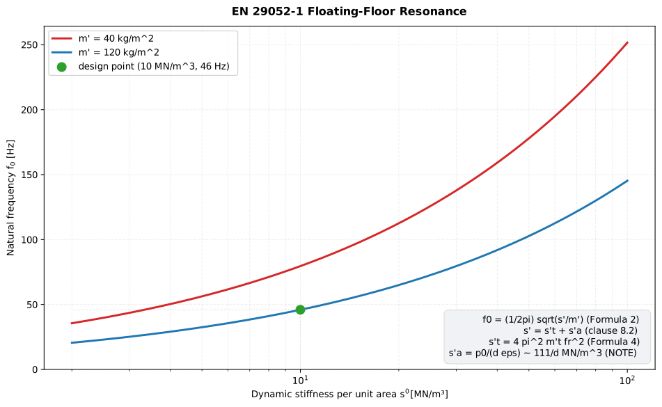
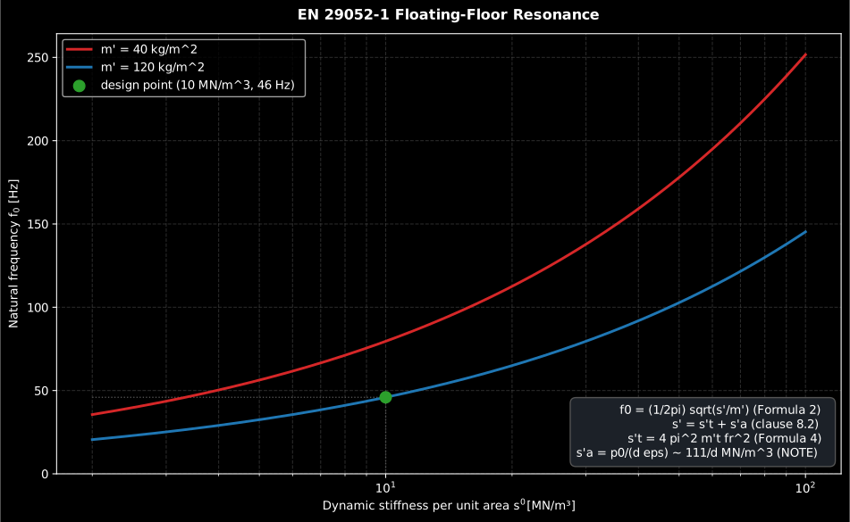
The whole design problem in one chart: $f_0=(1/2\pi )\sqrt{s^{\prime }/m^{\prime }}$, so the natural frequency falls as the square root of the layer’s dynamic stiffness and rises as the square root of one over the slab’s surface mass. Quartering $s^{\prime }$ halves $f_0$, and so does quadrupling the slab mass. A floating floor only improves insulation well above $f_0$, which is why the design goal is a soft layer under a heavy slab — and why the flat right-hand end of the curve means that a stiffer layer costs less than it looks.

Show the code for this figure

import matplotlib.pyplot as plt
import numpy as np
from phonometry import materials

# The design curve for a light and a heavy floating floor (Formula 2).
s = np.logspace(np.log10(2.0), np.log10(100.0), 300)   # MN/m3
for m in (40.0, 120.0):
    plt.semilogx(s, materials.natural_frequency(s * 1e6, m), label=f"m' = {m:g} kg/m²")
plt.xlabel("Dynamic stiffness s' [MN/m³]"); plt.ylabel("Natural frequency f₀ [Hz]")
plt.legend(); plt.show()

# A measured determination draws the same curve with its own point marked;
# `floating_floor_resonance` and its arguments are the subject of section 2.

1. Dynamic stiffness and resonance

The dynamic stiffness per unit area is a dynamic force per area divided by the resulting change in thickness (Formula 1): $s^{\prime }=(F/S)/\Delta d$. The resiliently supported floor is a resonator whose natural frequency (Formula 2) and, in the laboratory arrangement, measured resonant frequency (Formula 3) are

$$f_0=\frac{1}{2\pi }\sqrt{\frac{s^{\prime }}{m^{\prime }}},f_r=\frac{1}{2\pi }\sqrt{\frac{s_t^{\prime }}{m_t^{\prime }}},$$

so the apparent dynamic stiffness follows from the resonance (Formula 4):

$$s_t^{\prime }=4{\pi }^2{m}_t^{\prime }{f}_r^2.$$

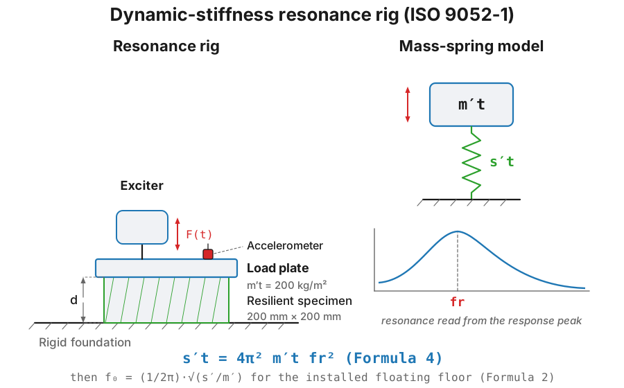
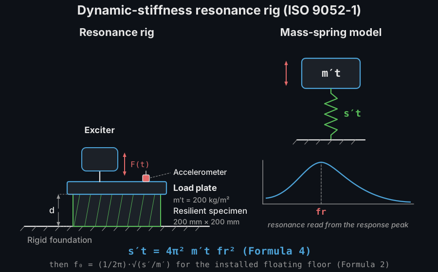
In the test arrangement the specimen lies between a base and a load plate whose total mass per unit area, plate plus added load, is 200 kg/m² (8 kg on the 0.04 m² specimen). That load reproduces the static preload of a typical floating floor, about 2 kPa, and it is why the standard’s scope stops at loadings below 0.4 kPa and above 4 kPa. A vertical exciter drives the system, an accelerometer picks up its response, and the fundamental vertical resonance $f_r$ of the plate-on-specimen system is read from the response peak; Formula 4 turns it into $s_t^{\prime }$.

1.1 Getting $f_r$

The library takes $f_r$ as an input, and Clause 7 is how a laboratory produces one. Three excitation signals are offered and declared equivalent: sinusoidal, white noise and pulse. Sinusoidal is the reference method in case of dispute; white-noise and pulse excitation are analysed as a frequency response per ISO 7626-2 or by impact excitation. The three arrangements drawn above differ in where the exciter sits and what is measured: on a rigid base whose velocity is negligible against the load plate’s, the load plate alone is enough; on a baseplate of at least 100 kg carried on soft mounts, both plates are measured. Whichever is used, the arrangement must permit vertical motion only, without rotational components, and it is reported with the result.

The sinusoidal procedure is a sweep at constant excitation force. The catch is that $f_r$ often depends on that force, because a resilient layer is non-linear: drive it harder and it softens, and the peak walks down in frequency. So the standard does not ask for a resonance, it asks for the resonance the material would have at vanishing amplitude:

1. Sweep at one force amplitude and read the peak.
2. Repeat at at least three force amplitudes inside the interval the expected stiffness selects: $0.2\text{N}\le F\le 0.8\text{N}$ for $s^{\prime }>50$ MN/m³, and $0.1\text{N}\le F\le 0.4\text{N}$ for $s^{\prime }\le 50$ MN/m³.
3. Extrapolate the $(F,f_r)$ points linearly to zero force. That intercept is the $f_r$ the library expects.

import numpy as np

# `materials` is imported by the block above. Three sinusoidal sweeps inside
# the 0.1-0.4 N interval (this layer is well under 50 MN/m3), each giving its
# own peak: the layer softens as it is driven harder, so f_r walks down.
force = np.array([0.10, 0.25, 0.40])          # N
peak = np.array([25.6, 25.0, 24.4])           # Hz, read from the response

slope, intercept = np.polyfit(force, peak, 1)
print(round(float(intercept), 2))             # 26.0  Hz at F -> 0
s_t = materials.apparent_dynamic_stiffness(resonant_frequency=intercept,
                                           total_mass_per_area=200.0)
print(round(s_t / 1e6, 3))                    # 5.337  MN/m3
# Taking the hardest-driven sweep at face value instead gives 4.701 MN/m3,
# 12 % low, and a floating-floor f0 about 5 % low with it.

One material defeats the peak-reading altogether. When the internal damping is high the vertical vibration maximum is not pronounced, and the standard’s answer is to stop looking at the magnitude: locate the resonance from the phase shift between the excitation and the vibration signal instead. That phase is not a fallback reading of the same thing — it is a sharper one, and watching a sweep run through $f_r$ shows why.

A sinusoidal sweep from 8 Hz to 60 Hz drives the 8 kg load plate on its resilient specimen while the response magnitude and phase are tracked. Below the 25 Hz resonance the plate moves in phase with the force; at resonance the amplitude peaks and the motion falls a quarter cycle behind, crossing minus 90 degrees; above it the plate moves against the force towards antiphase. The plate is watched stroboscopically at the drive frequency and its motion is drawn on a compressed amplitude scale, so what moves on screen is the phase relationship rather than the 25 Hz oscillation itself.

Download the animation (WebM)

A sinusoidal sweep from 8 Hz to 60 Hz drives the 8 kg load plate on its resilient specimen while the response magnitude and phase are tracked. Below the 25 Hz resonance the plate moves in phase with the force; at resonance the amplitude peaks and the motion falls a quarter cycle behind, crossing minus 90 degrees; above it the plate moves against the force towards antiphase. The plate is watched stroboscopically at the drive frequency and its motion is drawn on a compressed amplitude scale, so what moves on screen is the phase relationship rather than the 25 Hz oscillation itself.

Download the animation (WebM)

The magnitude peak is broad — it is what the loss factor makes of it — while the phase runs through $-90°$ steeply and crosses it at $f_r$ whatever the damping. That is the whole reason the standard offers the phase reading for damped materials, and it is worth having on any rig, because a peak that is 2 Hz wide is a peak that can be read 2 Hz wrong.

1.2 Preparing the specimen and the rig

The measured $f_r$ is decided by the bedding and by the rig tolerances at least as much as by the material, and both are normative.

• Specimens. At least three, each 200 mm × 200 mm (Clause 6). Their surfaces count as smooth only if the irregularities are under 3 mm.
• Bedding. Cover the specimen with a waterproof plastic foil about 0.02 mm thick, apply a thin paste of plaster of Paris and water at least 5 mm deep so that any unevenness is covered, and bed the load plate onto it before the plaster sets. A dry or partial contact carries the load on part of the specimen area, stiffens the reading and biases $f_r$ upward.
• Closed-cell materials. Seal the joint between the specimen and the base around the perimeter with a fillet of petroleum jelly. An unsealed perimeter changes what the enclosed gas of section 2 can do.
• Plates. The load plate is steel, (200 ± 3) mm square, and both it and the base have profile irregularities under 0.5 mm and are stiff enough to avoid bending waves in the frequency range of interest.
• The load is a budget, not a plate. The total load on the specimen is 8 kg ± 0.5 kg including all measuring and excitation equipment, so the accelerometer, the stinger and anything else resting on the plate count against it.

from phonometry import materials

# Standard 8 kg load plate on the 0.04 m2 specimen -> m't = 200 kg/m2;
# the fundamental resonance is measured at 25 Hz.
s_t = materials.apparent_dynamic_stiffness(resonant_frequency=25.0, total_mass_per_area=200.0)
print(round(s_t / 1e6, 3))                              # 4.935  MN/m3

# Installed on a 120 kg/m2 floating screed with s' = 10 MN/m3:
print(round(materials.natural_frequency(10e6, 120.0), 1))      # 45.9  Hz

That little oscillator is small enough to draw at true scale. plot_dynamic_stiffness_rig puts the standard 200 mm specimen under the 8 kg load plate with the exciter and accelerometer in place.

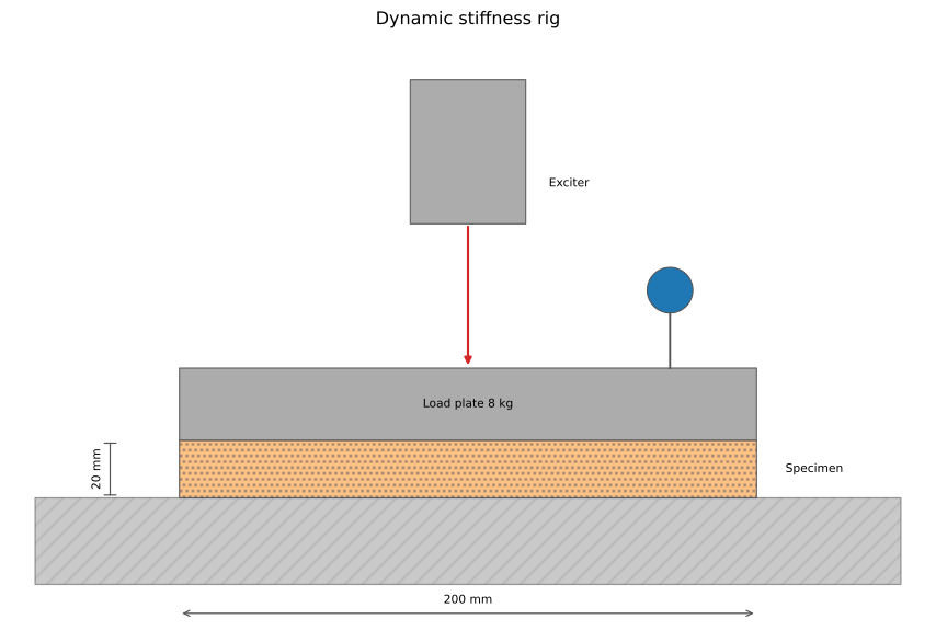
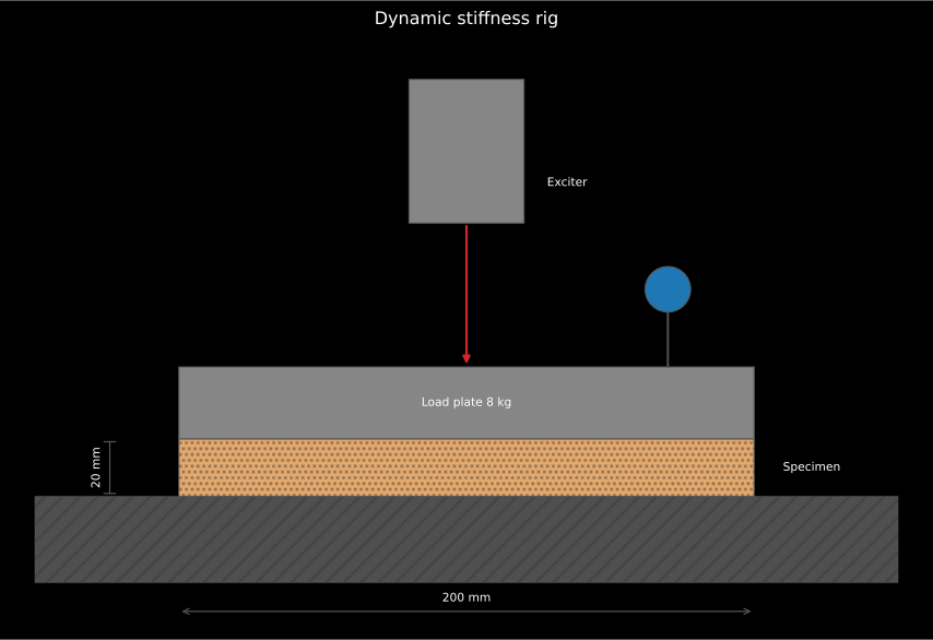
The mass-spring system behind $s^{\prime }$ at true scale: 20 mm of resilient layer under the 8 kg plate is all it takes to reproduce the 2 kPa preload of a floating floor.

Show the code for this figure

import matplotlib.pyplot as plt
from phonometry import materials

# The standard rig: a 200 mm square specimen under the 8 kg load plate.
materials.plot_dynamic_stiffness_rig()
plt.show()

2. The enclosed-gas term and airflow resistivity

For an air-permeable material the enclosed pore air adds a parallel stiffness from its isothermal compression (Formula 7): $s_a^{\prime }=p_0/(d\epsilon )$, with $p_0$ the atmospheric pressure, $d$ the loaded thickness and $\epsilon$ the porosity. The standard’s worked NOTE ($p_0=0.1\text{MPa}$, $\epsilon =0.9$) is $s_a^{\prime }=111/d$ MN/m³ for $d$ in millimetres:

from phonometry import materials

print(round(materials.enclosed_gas_stiffness(thickness=0.020, porosity=0.9) / 1e6, 2))
# 5.56  MN/m3   (the NOTE's 111/20 = 5.55 MN/m3)

That term is not a rounding correction. At 20 mm it is already larger than the frame stiffness the rig measured, and below about 22 mm the pore air, not the material, is the spring.

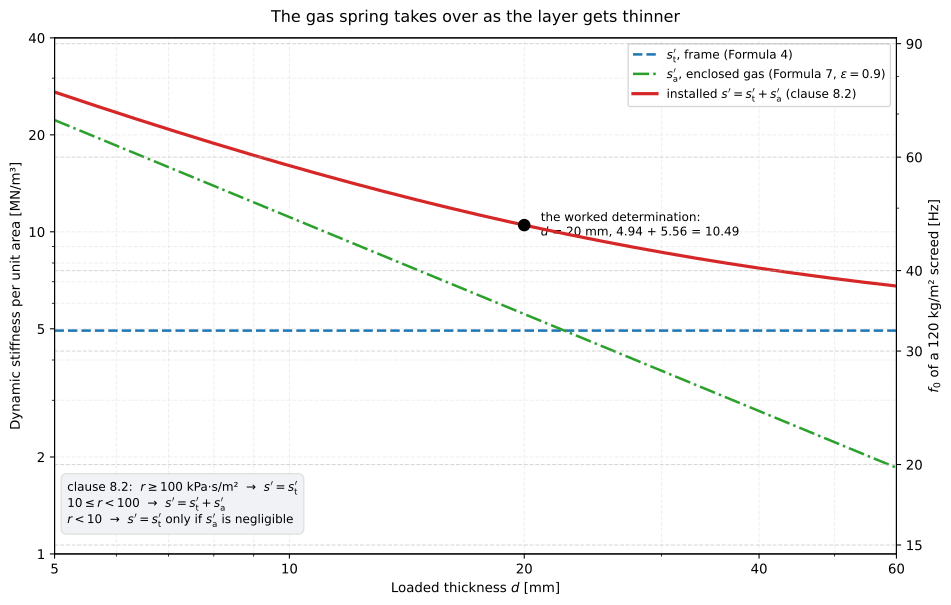
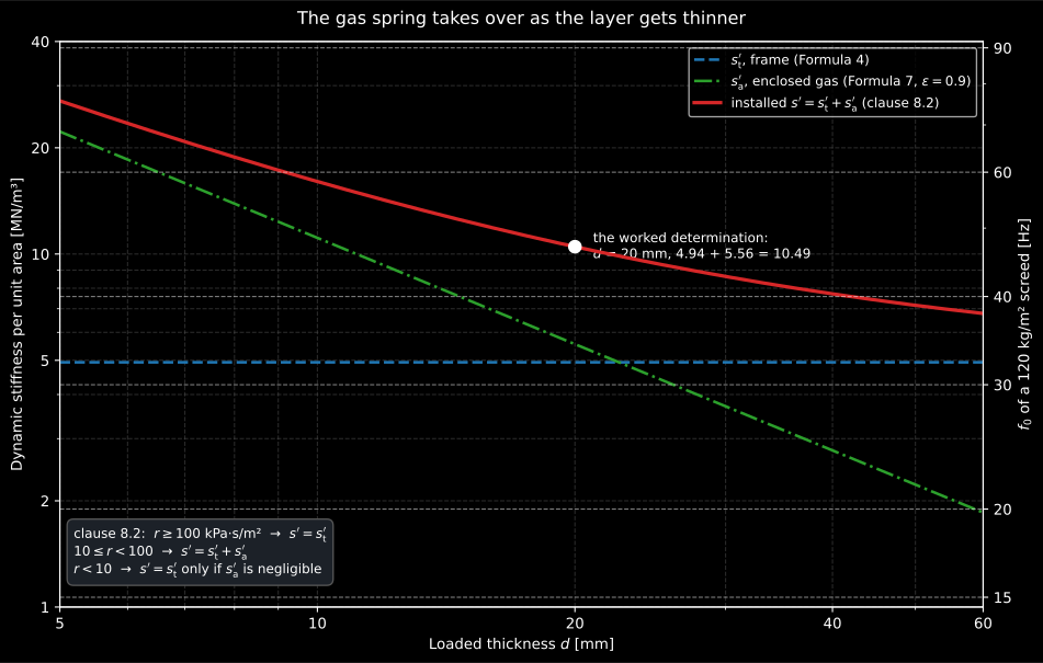
The inversion that decides whether a thin layer can ever be soft. The frame stiffness $s_t^{\prime }$ is a property of the material and does not care how thick the layer is; the enclosed-gas term $s_a^{\prime }=p_0/(d\epsilon )$ does, and it grows without limit as the layer thins. Below the crossing near 22 mm the air in the pores is the stiffer of the two springs, so a 10 mm permeable layer cannot be soft however soft its frame is: 11 MN/m³ of gas alone puts $f_0$ back above 50 Hz on a 120 kg/m² screed. The right-hand axis is the same $s^{\prime }$ read as that natural frequency.

Show the code for this figure

import matplotlib.pyplot as plt
import numpy as np

# `materials` is imported above. The clause 8.2 sum against loaded thickness,
# the frame term held at the worked determination's 4.94 MN/m3.
d_mm = np.logspace(np.log10(5.0), np.log10(60.0), 300)
s_gas = np.array([materials.enclosed_gas_stiffness(thickness=d * 1e-3,
                                                   porosity=0.9) / 1e6
                  for d in d_mm])
fig, ax = plt.subplots()
ax.loglog(d_mm, np.full_like(d_mm, 4.935), "--", label="s't, frame")
ax.loglog(d_mm, s_gas, "-.", label="s'a, enclosed gas")
ax.loglog(d_mm, 4.935 + s_gas, "-", label="s' installed")
ax.set_xlabel("Loaded thickness d [mm]")
ax.set_ylabel("Dynamic stiffness per unit area [MN/m³]")
ax.legend()
plt.show()

The dynamic stiffness of the installed material is then set by the lateral airflow resistivity $r$ (clause 8.2): $s^{\prime }=s_t^{\prime }$ for $r\ge 100\text{kPa}\cdot {\text{s/m}}^2$, $s^{\prime }=s_t^{\prime }+s_a^{\prime }$ for $10\le r<100\text{kPa}\cdot {\text{s/m}}^2$, and for $r<10\text{kPa}\cdot {\text{s/m}}^2$ the method only resolves $s^{\prime }=s_t^{\prime }$ when the gas term is negligible.

Why lateral resistivity decides anything. Under the load plate the layer is compressed, and the pore air has two ways out: it can be squeezed sideways out of the layer, or it can be compressed in place with the frame. It is a spring in parallel with the frame only in the second case, and the lateral airflow resistivity is exactly what decides which happens. That maps onto the three branches. At high $r$ the air is trapped both in the 200 mm specimen and under a full floor, so the $s_t^{\prime }$ the rig measured already contains it and nothing is added. At intermediate $r$ it escapes from the small specimen but not from a floor several metres across, so the standard computes $s_a^{\prime }$ and adds it back. At low $r$ it escapes from both: there is no gas spring to add, but the method can no longer separate the two contributions either. In that third case report $s^{\prime }=s_t^{\prime }$ with the reservation, and state the estimated error of disregarding $s_a^{\prime }$ — the standard asks for exactly that. Note also where $r$ comes from: it is the same viscous property ISO 9053 measures, but along the layer rather than through it, and here it is an input rather than something the method determines. Take the porosity $\epsilon$ for $s_a^{\prime }$ as the standard’s 0.9 unless it has been measured.

Mind the prefix. $r$ is the quantity ISO 9053 calls $\sigma$ and reports in Pa·s/m², while EN 29052-1 writes it $r$ and thresholds it in kPa·s/m². The library follows the standard, so airflow_resistivity is in kPa·s/m² — the one argument on this page that is not plain SI. A mineral wool measured at 50 000 Pa·s/m² goes in as 50.0, not 50000.0; convert an ISO 9053 result with sigma / 1000. Passing the Pa·s/m² number lands silently in the $r\ge 100$ branch, which drops the enclosed-gas term: for the determination below that turns $s^{\prime }=10.49$ MN/m³ into 4.93 MN/m³ and the design natural frequency from 47.1 Hz to 32.3 Hz, with no warning, because the wrong branch is a valid branch.

floating_floor_resonance chains the whole determination:

from phonometry import materials

res = materials.floating_floor_resonance(
    resonant_frequency=25.0, total_mass_per_area=200.0,
    floor_mass_per_area=120.0,
    airflow_resistivity=50.0,   # kPa.s/m2 (= 50000 Pa.s/m2 from ISO 9053)
    thickness=0.020, porosity=0.9,
)
print(round(res.dynamic_stiffness / 1e6, 2), round(res.natural_frequency, 1))
# 10.49 47.1

res.plot()   # the f0(s') design curve with this determination marked (needs matplotlib)

The DynamicStiffnessResult carries the apparent, enclosed-gas and installed stiffnesses, the test resonance and the installed-floor natural frequency, and its .plot() draws the $f_0(s^{\prime })$ design curve.

Test-report fiche

DynamicStiffnessResult.report(path) renders a one-page accredited dynamic-stiffness test report (EN 29052-1:1992 = ISO 9052-1:1989): a metadata header (specimen, the total mass per unit area $m_t^{\prime }$ used during the test, the loaded thickness $d$ (in metres, shown in mm), test facility, climate), a compact metrics table (the resonant frequency $f_r$, the apparent stiffness $s_t^{\prime }$ of Formula 4, the enclosed-gas term $s_a^{\prime }$ when it applies, the installed $s^{\prime }$ of clause 8.2 and the natural frequency $f_0$ of Formula 2) beside the $f_0(s^{\prime })$ design curve, and a boxed apparent dynamic stiffness $s_t^{\prime }$ with the installed $s^{\prime }$ and the resonance $f_r$ alongside. Clause 9 rounds every stiffness to the nearest MN/m³. It is a characterisation, so there is no pass/fail verdict; language="es" renders the Spanish fiche. The fiche always embeds the $f_0(s^{\prime })$ design curve, so it needs both the report and plot extras (pip install "phonometry[report,plot]").

from phonometry import ReportMetadata, materials

res = materials.floating_floor_resonance(
    resonant_frequency=45.0, total_mass_per_area=200.0,
    floor_mass_per_area=110.0,
    airflow_resistivity=50.0,   # kPa.s/m2 (= 50000 Pa.s/m2 from ISO 9053)
    thickness=0.020, porosity=0.9,
)
res.report(
    "dynamic_stiffness.pdf",
    metadata=ReportMetadata(
        specimen="20 mm mineral-wool resilient layer",
        mass_per_area=200.0, thickness=0.020,   # thickness d in metres (20 mm)
        measurement_standard="EN 29052-1",
    ),
)   # one-page fiche (needs phonometry[report,plot])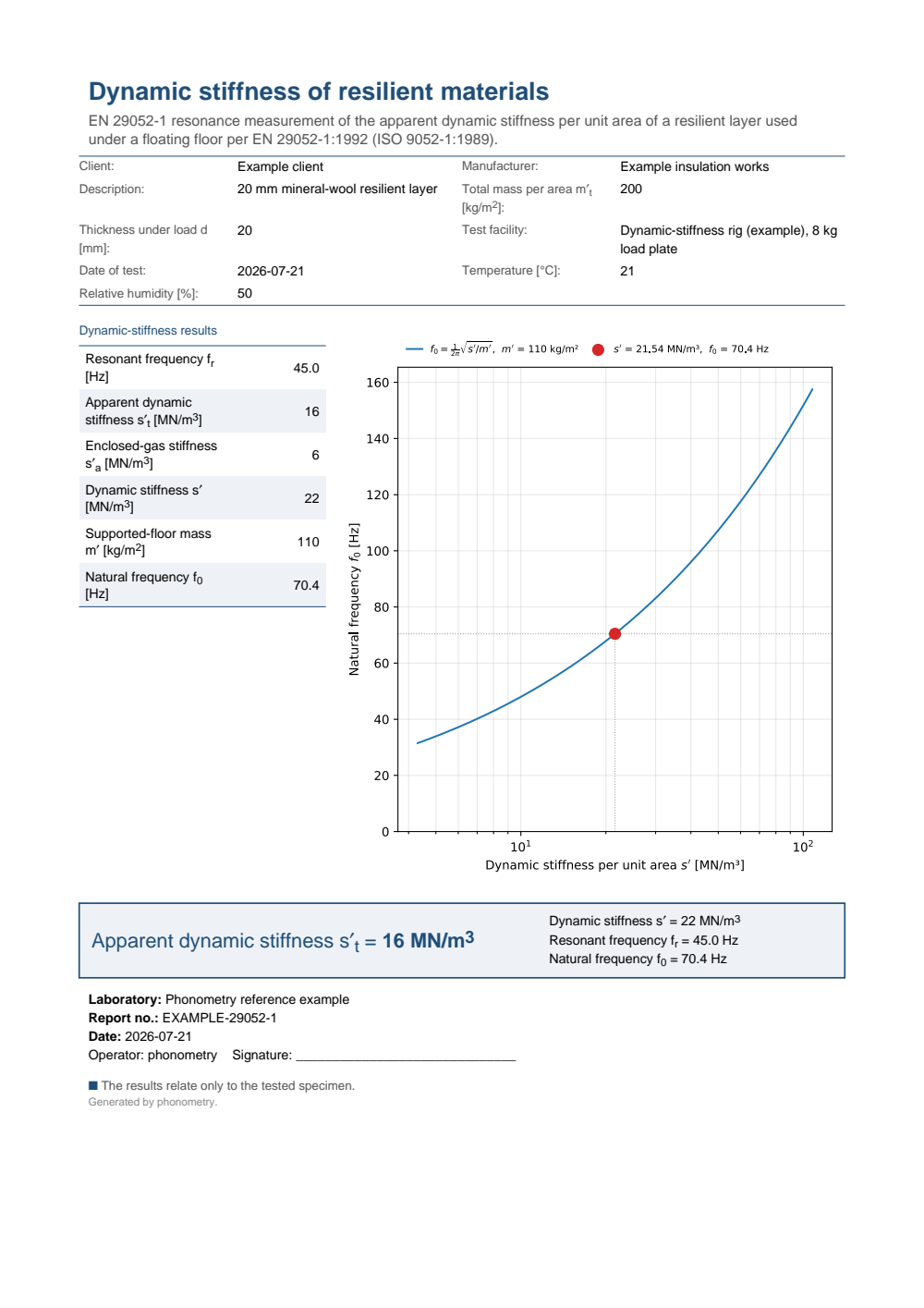

One-page dynamic-stiffness fiche: a metadata header with the total mass per unit area and the loaded thickness, a metrics table of the resonant frequency, the apparent, enclosed-gas and installed dynamic stiffnesses and the natural frequency beside the f0(s') design curve, and the boxed apparent dynamic stiffness s't.

Download the report (PDF)

Dynamic-stiffness fiche (DynamicStiffnessResult.report): the resonance metrics and the f0(s') design curve.

3. What the resonance method assumes, and where it bites

The evaluation treats the rig as a single-degree-of-freedom system: the load plate moves as a rigid piston on a massless spring. That holds while the specimen is light against the plate and its first internal resonance sits well above $f_r$; a heavy or very thick layer starts to act as a distributed system and the simple Formula 4 reading degrades. Three practical pitfalls follow from the preload:

• $s^{\prime }$ is a stiffness at the standard preload. Resilient layers are visibly non-linear in static load: mineral wool stiffens as it compresses, some foams soften. The 200 kg/m² load plate fixes the operating point, so the tabulated $s^{\prime }$ strictly describes floors near that surface mass. Designing a much heavier screed with the same $s^{\prime }$ extrapolates beyond the measurement.
• Drive small. The tangent stiffness is defined for small dynamic strains; driving the plate hard pushes the layer into its non-linear range and shifts the apparent resonance downward. Keep the excitation at the lowest level that gives a clean peak.
• Respect the contact. The standard seats the load plate on a thin bonding layer (a plaster paste) so the full specimen area carries the load. A dry, uneven contact concentrates the force, stiffens the response locally and biases $f_r$ upward.

3.1 Reading $s^{\prime }$, and what it buys

The natural frequency that matters in the end is not the rig’s $f_r$ but the installed floor’s $f_0$ from Formula 2. Two questions follow, and the page owes both an answer.

Is 10.5 MN/m³ a good number? Resilient layers used under screeds run from a few MN/m³ for soft elastomeric products and low-density mineral wools up to several tens for stiffer boards, so the worked determination sits in the middle of the usable range. The floor under it is the enclosed-gas term: for a 90 % porous layer it alone contributes about $111/d$ MN/m³ with $d$ in millimetres, so a thin permeable layer cannot be soft whatever its frame does.

What does a low $f_0$ buy? The floating floor improves impact insulation by $\Delta L=30\lg (f/f_0)$ for sand-cement and calcium-sulfate screeds (ISO 12354-2 Formula (C.1)), and by $40\lg (f/f_0)$ for asphalt and dry floors. So the 47 Hz of the worked determination gives about 31 dB at 500 Hz and nothing at all at and below $f_0$ — and halving $f_0$ buys roughly 9 dB across the whole band, which is why the entire method exists. The practical target is to keep $f_0$ below the lowest band of interest.

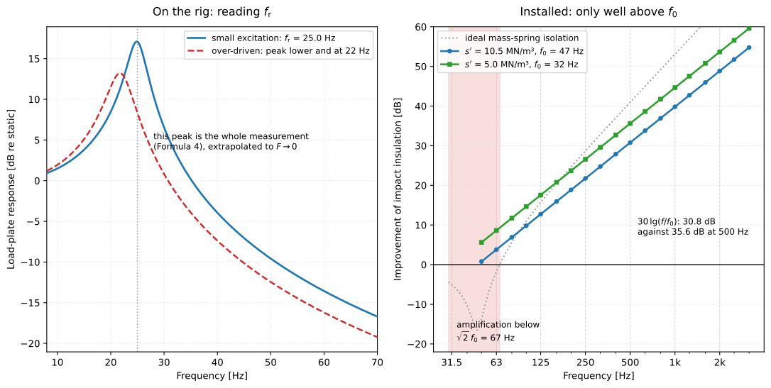
Left: the peak the operator reads off the rig, and what over-driving does to it — the resonance walks down in frequency and flattens, which is the whole reason for the extrapolation of section 1.1. Right: what the installed floor does with the result. Nothing is gained below $\sqrt{2}{f}_0$; the shaded region is where an undamped mass-spring floor would be worse than no floating floor at all, and the ISO 12354-2 law truncates that to zero rather than predicting the ideal peak, because a real screed on a real layer is damped. Halving $s^{\prime }$ moves $f_0$ down by $\sqrt{2}$ and lifts the whole curve by about 5 dB — 30.8 dB against 35.6 dB at 500 Hz for the two layers drawn.

Show the code for this figure

import matplotlib.pyplot as plt
import numpy as np

# `materials` is imported above. The ISO 12354-2 law in closed form for the
# worked determination and for a layer half as stiff; the library evaluates
# the same law, with its branches, in floating_floor_improvement_spectrum
# (see the resilient-layer prediction guide).
bands = np.array([50, 63, 80, 100, 125, 160, 200, 250, 315, 400, 500,
                  630, 800, 1000, 1250, 1600, 2000, 2500, 3150], float)
fig, ax = plt.subplots()
for stiffness in (10.49e6, 5.0e6):
    f0 = float(materials.natural_frequency(stiffness, 120.0))
    delta_l = np.maximum(30.0 * np.log10(bands / f0), 0.0)   # Formula (C.1)
    ax.semilogx(bands, delta_l, "o-", label=f"f0 = {f0:.0f} Hz")
ax.set_xlabel("Frequency [Hz]")
ax.set_ylabel("Improvement of impact insulation [dB]")
ax.legend()
plt.show()

How much improvement that actually buys band by band, and what it becomes as a weighted single number, is Predicting Resilient-Layer Performance.

What this guide covers

• Covered

  EN 29052-1:1992 (identical to ISO 9052-1:1989) for materials under floating floors: the dynamic stiffness per unit area of Formula 1, the resonance relations of Formulae 2-4 (apparent_dynamic_stiffness, natural_frequency), the enclosed-gas term of Formula 7 (enclosed_gas_stiffness), and the clause 8.2 airflow-resistivity regimes of Formulae 5-6 (installed_dynamic_stiffness), chained end to end by floating_floor_resonance. DynamicStiffnessResult.report renders the clause 9 test-report fiche.

• Not covered

  Clause 7’s measurement procedure, extracting the resonant frequency $f_r$ from the raw excitation-response signal by sinusoidal, white-noise or pulse methods, is not implemented: pass an already-extrapolated $f_r$, obtained as section 1.1 describes (the extrapolation itself is a straight-line fit, which section 1.1 shows). The lateral airflow resistivity $r$ of clause 8.2 is likewise taken as an input rather than measured; ISO 9053’s static and alternating methods are implemented separately, in materials.absorbers.airflow_resistance, and they report $\sigma$ in Pa·s/m² while this page’s airflow_resistivity argument is in kPa·s/m². Clause 6’s specimen-selection requirement (at least three 200 mm × 200 mm specimens) is not enforced, and neither is the Clause 9 report content: the fiche below carries the excitation arrangement and the signal type only if they are supplied in the metadata.

See also

• Predicting Resilient-Layer Performance: what the design side does with $s^{\prime }$, from the mass-spring resonance to the improvement laws above it and their weighted single number.
• Predicting Sound Insulation (EN 12354): the floating-floor term this measurement feeds.
• Airflow Resistance: the ISO 9053 determination of the lateral resistivity $r$ that clause 8.2 needs, reported there as $\sigma$ in Pa·s/m².
• Resilient layers overview: where this measurement sits among the materials guides.
• API reference: materials.resilient.dynamic_stiffness.
• Theory: Point mobilities and radiation efficiency: the mass-spring resonance the EN 29052-1 rig measures, seen as a mobility.

References

• International Organization for Standardization. (1989). Acoustics — Determination of dynamic stiffness — Part 1: Materials used under floating floors in dwellings (EN 29052-1:1992 (ISO 9052-1:1989)). EN 29052-1:1992 is the identical European adoption of ISO 9052-1:1989 and is the designation this page uses throughout; the ISO URL is the citable one. The method implemented here: the dynamic stiffness per unit area (Formula 1), the resonance relations (Formulae 2-4), the enclosed-gas term (Formula 7, clause 8.2 NOTE s'a = 111/d MN/m³) and the airflow-resistivity regimes (Formulae 5-6). Conformance is anchored on the standard's own numeric NOTE plus hand-computed closed-form values of the resonance relations.
• Vigran, T. E. (2008). Building acoustics. CRC Press. https://doi.org/10.1201/9781482266016Floating-floor design and the role of the resilient layer's dynamic stiffness in the impact-sound improvement. ISBN 978-0-415-42853-8.