Predicting Resilient-Layer Performance

A resilient layer is the cheapest way to buy impact sound insulation and the easiest to get wrong. Whether it is a carpet on a slab, a screed floating on mineral wool or a plasterboard lining on a masonry wall, the layer is a spring, and the only question that matters is where its resonance with the mass it carries falls. Below that frequency it does nothing, at it the construction is worse than bare, and above it the improvement climbs at a rate the construction type decides. This guide is the prediction side of that story, from the material data to the improvement spectrum; the measurement side lives in Floor-Covering Impact Improvement (ISO 16251-1) and Dynamic stiffness of resilient materials.

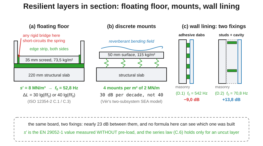
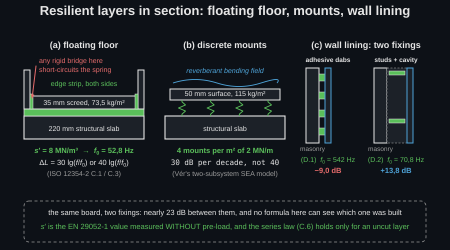
Every formula below is chosen by a construction detail, so it is worth having the three build-ups in view: a continuous resilient layer under a screed, discrete mounts under a walking surface, and a lining fixed to a wall either by bonding or on studs over a cavity. Which of them you have built decides which law applies — and, as the last section of this page shows, whether the prediction means anything at all.

The excitation: the tapping machine as a mass-spring-dashpot

Everything downstream depends on the force the standard tapping machine actually injects, and that force is not a property of the machine alone. Each hammer is a 0.5 kg mass dropped 40 mm, so it lands at $v_{\text{h}}=\sqrt{2gh}=0.886\text{m/s}$, ten times a second. If the impact were short compared with the 0.1 s between impacts, the momentum alone would fix the force, giving the line spectrum $|F_n|=2m{v}_{\text{h}}/T_i$ and the band mean-square force $F_{\text{rms}}^2=3.9B$ that ISO 10140 measurements on concrete are usually reduced with.

Real floors deform. The hammer, the contact stiffness $K$ it presses into and the floor’s driving-point impedance $Z_{\text{dp}}$ form a mass-spring-dashpot whose pulse splits into two cases:

• over-critical, $Km\ge 4Z_{\text{dp}}^2$: a single positive pulse, no rebound. This is a lightweight walking surface (chipboard, OSB), where the spectrum tends to $|F_n{|}_{\text{lower}}=m{v}_{\text{h}}/T_i$;
• under-critical, $Km<4Z_{\text{dp}}^2$: the hammer rebounds and only the first positive lobe counts. This is a concrete slab or a screed, where the spectrum sits within 1 dB of $|F_n{|}_{\text{upper}}=2m{v}_{\text{h}}/T_i$ below 4 kHz and the short-pulse estimate is adequate.

The two limits are 6 dB apart in mean square, which is the whole reason a tapping-machine level on a timber floor cannot be compared with one on concrete without thinking. Above the cut-off frequency

$$f_{\text{co}}=\frac{1}{2\pi }\sqrt{\frac{K}{m}}\text{(under-critical)},f_{\text{co}}=\frac{1}{2\pi }\left[\frac{K}{2Z_{\text{dp}}}-\sqrt{{\left(\frac{K}{2Z_{\text{dp}}}\right)}^2-\frac{K}{m}}\right]\text{(over-critical)},$$

the force falls away, and above the limiting frequency $f_{\text{limit}}=Z_{\text{dp}}/(2\pi m)$ the hammer’s own mass impedance, not the floor, caps the injected power.

import numpy as np
from phonometry import (
    hammer_impact_velocity, infinite_plate_impedance, plate_bending_stiffness,
    plate_contact_stiffness, tapping_force_spectrum,
)

print(round(hammer_impact_velocity(), 3))     # 0.886 m/s (0.5 kg dropped 40 mm)

# A 140 mm cast in-situ concrete slab: 2200 kg/m3, cL = 3800 m/s, nu = 0.2.
rho, c_l, nu, h = 2200.0, 3800.0, 0.2, 0.14
E = rho * c_l**2 * (1 - nu**2)
z = infinite_plate_impedance(plate_bending_stiffness(E, h, nu), rho * h)
k = plate_contact_stiffness(E, poisson_ratio=nu)

freqs = np.array([100, 200, 400, 800, 1600, 3150], dtype=float)
res = tapping_force_spectrum(freqs, k, z)
res.over_critical            # False: the hammer rebounds off concrete
round(res.cut_off_frequency)  # 6948 Hz, above the building acoustics range
res.peak_force               # |Fn| per band, within 1 dB of res.upper_limit
res.power_input_level        # 10 lg(Win/1 pW), rising 3 dB per doubling
res.plot()                   # the force spectrum with both asymptotes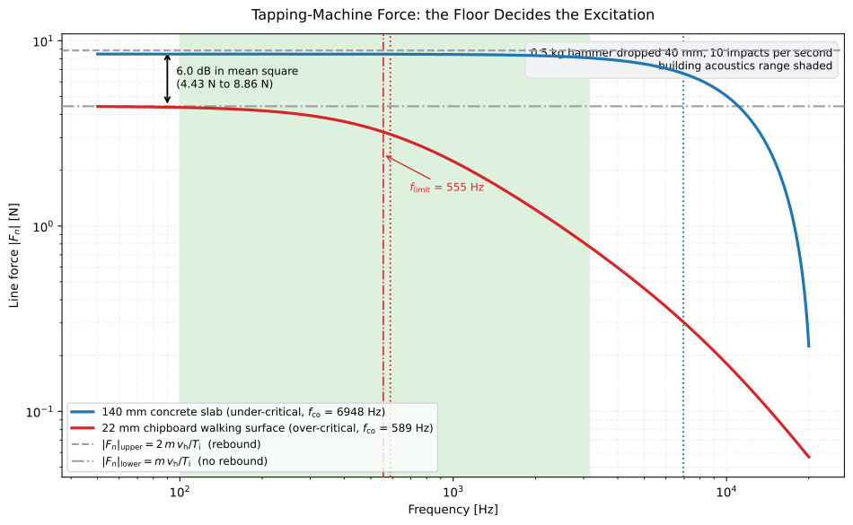

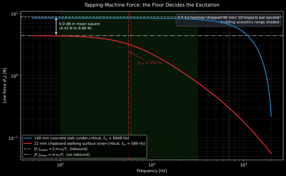
The same machine, two floors. On concrete the hammer rebounds (under-critical) and the spectrum hugs the upper asymptote $|F_n{|}_{\text{upper}}=2m{v}_{\text{h}}/T_i$ to within 1 dB right across the building acoustics range, its cut-off sitting at 6 948 Hz and its hammer limiting frequency at 120 kHz — both far outside anything that is rated. On 22 mm chipboard the surface gives way, the hammer does not rebound (over-critical), and both frequencies collapse into the middle of the range: $f_{\text{co}}$ = 589 Hz and $f_{\text{limit}}$ = 555 Hz, so the spectrum bends towards the lower asymptote $m{v}_{\text{h}}/T_i$ where a rated band actually sits. The two asymptotes are 6.0 dB apart in mean square, and that gap is the whole reason a tapping-machine level measured on a timber floor cannot be compared with one measured on concrete: the machine is injecting a different force.

Show the code for this figure

import matplotlib.pyplot as plt
import numpy as np
# The names come from the import block above.

freqs = np.logspace(np.log10(50.0), np.log10(20000.0), 400)
fig, ax = plt.subplots()
for label, rho_s, c_s, nu_s, h_s in (("140 mm concrete", 2200.0, 3800.0, 0.2, 0.14),
                                     ("22 mm chipboard", 650.0, 2400.0, 0.3, 0.022)):
    e_s = rho_s * c_s**2 * (1 - nu_s**2)
    z_s = infinite_plate_impedance(plate_bending_stiffness(e_s, h_s, nu_s),
                                   rho_s * h_s)
    k_s = plate_contact_stiffness(e_s, poisson_ratio=nu_s)
    r = tapping_force_spectrum(freqs, k_s, z_s)
    ax.loglog(freqs, r.peak_force, label=f"{label} (fco = {r.cut_off_frequency:.0f} Hz)")
    ax.axhline(r.upper_limit, ls="--", lw=0.8)
    ax.axhline(r.lower_limit, ls=":", lw=0.8)
ax.set(xlabel="Frequency [Hz]", ylabel="Line force $|F_n|$ [N]")
ax.legend()
plt.show()

Soft floor coverings: the cut-off frequency is the design

A soft covering on a heavyweight floor changes nothing but the force input: its mass is negligible and it barely touches the slab’s loss factor or bending stiffness. So its improvement is simply the ratio of the two force spectra,

$$\Delta L=20{\log }_{10}\frac{|F_n{|}_{\text{without}}}{|F_n{|}_{\text{with}}}\text{dB},$$

and the whole design collapses to one number, the covering’s own cut-off frequency, set by its contact stiffness $K=E\pi r^2/d$ with the hammer radius $r=15$ mm. Below $f_{\text{co}}$ the covering does nothing; above it the improvement rises at 12 dB per octave. Two straight lines are therefore a usable estimate, and thickening a homogeneous covering lowers $f_{\text{co}}$ and buys improvement everywhere above it.

One detail decides whether the numbers are usable. The tapping machine excites a line spectrum, at multiples of the 10 Hz impact rate, so the formula above is a statement about one Fourier component; a band value is the ratio of the band mean-square forces over the lines the band contains. The difference is not cosmetic: the model’s transform has exact nulls at odd multiples of $f_{\text{co}}$, so a band centre landing on one reads tens of dB high. With the 100 Hz cut-off below, the single line at 500 Hz gives 66.8 dB against a design estimate of 27.9 dB, while the band value is 33.3 dB. improvement is the band value; line_improvement is the per-line ratio, and carries the nulls where they belong.

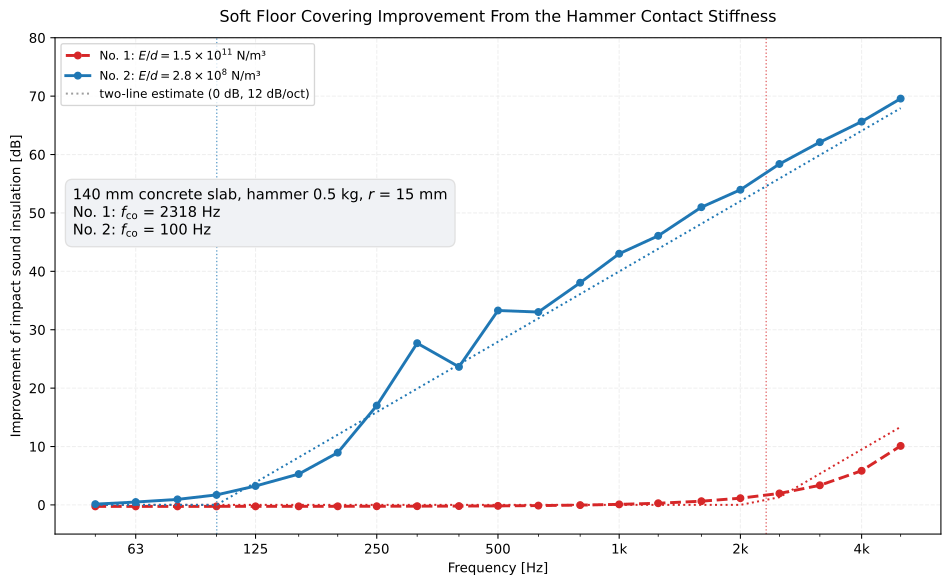
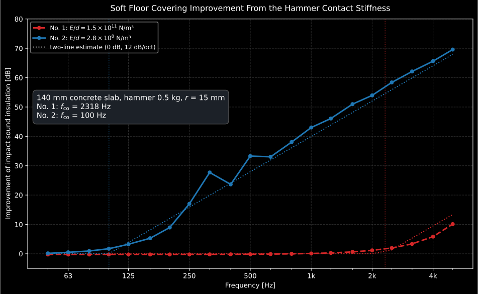
Two 5 mm coverings on the same slab, differing only in modulus, and the whole distance between them is $f_{\text{co}}$. The stiff PVC puts it at 2318 Hz, above most of the rating range, so it is still worth 3.4 dB at 3150 Hz and buys nothing where footfall lives; the resiliently backed one at 100 Hz is already worth 17.0 dB at 250 Hz and reaches 69.6 dB at 5 kHz. Above $f_{\text{co}}$ both climb at 12 dB per octave, and the dotted two-line construction tracks the band values within about 3 dB except around the transform’s nulls, where the 315 Hz band runs 7.8 dB high.

Show the code for this figure

import matplotlib.pyplot as plt
import numpy as np
from phonometry import (
    covering_contact_stiffness, covering_improvement, infinite_plate_impedance,
    plate_bending_stiffness, plate_contact_stiffness,
)

rho, c_l, nu, h = 2200.0, 3800.0, 0.2, 0.14          # 140 mm concrete slab
E = rho * c_l**2 * (1 - nu**2)
z = infinite_plate_impedance(plate_bending_stiffness(E, h, nu), rho * h)
plate = plate_contact_stiffness(E, poisson_ratio=nu)

bands = np.array([50, 63, 80, 100, 125, 160, 200, 250, 315, 400, 500, 630,
                  800, 1000, 1250, 1600, 2000, 2500, 3150, 4000, 5000.0])

d = 0.005
for label, modulus_over_thickness in (("PVC", 1.5e11), ("backed vinyl", 2.8e8)):
    res = covering_improvement(
        bands, covering_contact_stiffness(modulus_over_thickness * d, d),
        plate, z)
    plt.semilogx(bands, res.improvement, marker="o",
                 label=f"{label}: fco = {res.cut_off_frequency:.0f} Hz")
    plt.semilogx(bands, res.two_line, ":")
plt.legend()
plt.show()

from phonometry import covering_contact_stiffness, covering_improvement

# Covering No. 2 of Hopkins Fig. 4.64: E/d = 2.8e8 N/m3, a vinyl or carpet
# with a resilient backing, 5 mm thick on the same 140 mm slab.
d = 0.005
covering = covering_contact_stiffness(2.8e8 * d, d)
res = covering_improvement([125.0, 250.0, 500.0, 1000.0], covering, plate, z)
round(res.cut_off_frequency)        # 100 Hz
round(res.bare_cut_off_frequency)   # 6948 Hz, the bare slab's own cut-off
res.improvement                     # 3.2, 17.0, 33.3, 43.0 dB, band values
res.two_line                        # 3.9, 15.9, 27.9, 40.0 dB, the estimate
res.line_improvement                # per Fourier line, nulls at 3, 5, 7 fco
res.plot()

The model treats the covering as a linear spring. Under the tapping machine’s high force many real coverings harden, showing two or three slopes between 5 and 22 dB per octave rather than one, which is why a laboratory $\Delta L$ remains the reference once a specimen exists.

Floating floors: three laws above one resonance

A floating floor is a rigid walking surface on a resilient layer, and its resonance follows from the two numbers known at the drawing stage, the mass per unit area $m^{\prime }$ of the slab and the EN 29052-1 dynamic stiffness per unit area $s^{\prime }$ of the layer:

$$f_0=160\sqrt{\frac{s^{\prime }}{m^{\prime }}}\text{Hz}(s^{\prime }{\text{in MN/m}}^3,m^{\prime }{\text{in kg/m}}^2),$$

where 160 is the standard’s rounding of $1000/2\pi$. Above it, which law applies is a question about damping, not about the layer:

Model	Law	When
"cremer"	$\Delta L=40{\log }_{10}(f/f_0)$	Cremer’s infinite-plate result; asphalt screeds and dry floating floors, whose internal losses are high enough to behave as infinite plates (ISO 12354-2 Formula C.3). The derivation is reported to hold over $f_0<f<4f_0$, so the branch far above resonance is an extrapolation
"en12354"	$\Delta L=30{\log }_{10}(f/f_0)$	sand-cement and calcium-sulfate screeds, whose low loss factor makes them finite plates with a reverberant bending field (Formula C.1)
"cremer_hammer"	$40{\log }_{10}(f/f_0)+10{\log }_{10}[1+(f/f_{\text{limit}}{)}^2]$	a lightweight walking surface, where the hammer impedance is no longer negligible; tends to 18 dB per octave

All three laws are written for $f>f_0$, and the library clamps them to zero at and below the resonance. That clamp is a convention, not a physical result: in the band containing $f_0$ the mass-spring system amplifies, and measured floors fall between about $-5$ dB and $0$ dB there — the “worse than bare at $f_0$” of the introduction, which no model on this page reproduces. As long as $f_0$ sits below the rated range the difference is harmless, but a stiff layer or a light screed that puts $f_0$ near 100 Hz produces a $\Delta L_w$ that is optimistic in precisely the band that decides the rating. Check where $f_0$ lands before trusting the number.

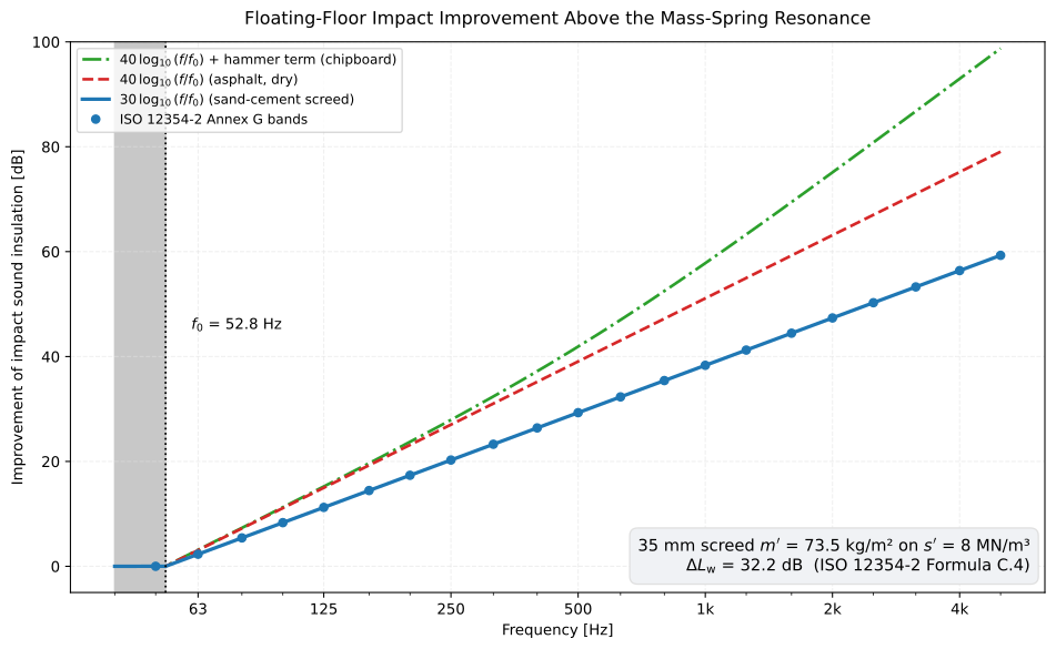
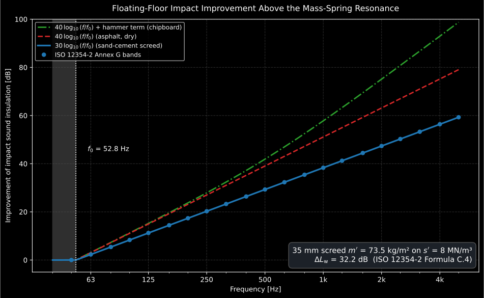
Identical $s^{\prime }$ and $m^{\prime }$, identical 52.8 Hz resonance, nothing below it — and three answers that part company immediately above: at 1 kHz 38.3, 51.1 and 57.8 dB, at 5 kHz 59.3, 79.1 and 98.7 dB. Choosing the branch is choosing the answer, and the choice is a statement about the screed’s internal damping and the walking surface’s impedance, not about the resilient layer, which is the same in all three.

Show the code for this figure

import matplotlib.pyplot as plt
import numpy as np
from phonometry import (
    floating_floor_improvement_spectrum, floating_floor_resonance_frequency,
)

# The worked floating floor of ISO 12354-2:2017 Annex G.
f0 = floating_floor_resonance_frequency(8.0e6, 73.5)     # 52.8 Hz
freqs = np.logspace(np.log10(40.0), np.log10(5000.0), 400)
for model, kwargs in (("en12354", {}), ("cremer", {}),
                      ("cremer_hammer", {"limiting_frequency": 521.0})):
    res = floating_floor_improvement_spectrum(
        freqs, resonance_frequency=f0, model=model, **kwargs)
    plt.semilogx(freqs, res.improvement, label=model)
plt.axvline(f0, ls=":")
plt.legend()
plt.show()

from phonometry import (
    combined_dynamic_stiffness, double_floating_floor_resonances,
    floating_floor_improvement_spectrum, floating_floor_resonance_frequency,
    weighted_floating_floor_improvement,
)

# 35 mm screed, m' = 73.5 kg/m2, on a resilient layer of s' = 8 MN/m3.
f0 = floating_floor_resonance_frequency(8.0e6, 73.5)
round(f0, 1)                                                    # 52.8 Hz

bands = [50, 63, 80, 100, 125, 160, 200, 250, 315, 400, 500, 630,
         800, 1000, 1250, 1600, 2000, 2500, 3150, 4000, 5000.0]
res = floating_floor_improvement_spectrum(
    bands, resonance_frequency=f0, mass_per_area=73.5, dynamic_stiffness=8.0e6)
res.improvement          # 0.0, 2.3, 5.4, 8.3, 11.2 ... 59.3 dB
round(res.delta_lw, 1)   # 32.2 dB, the Formula (C.4) weighted improvement
res.plot()

# Two resilient layers act as springs in series (Formula C.6), which drops the
# resonance by sqrt(2) and buys about 4.5 dB everywhere above it.
round(floating_floor_resonance_frequency(
    combined_dynamic_stiffness([8.0e6, 8.0e6]), 73.5), 1)       # 37.3 Hz

# One floating floor on top of another has two resonances instead of one; the
# adverse dip disappears, but the steep rise only starts above the higher.
double_floating_floor_resonances(7.25e6, 12.78, 7.25e6, 12.78)  # (74, 194) Hz

The weighted single numbers come straight from the same two inputs, so a floating floor can be sized without ever drawing a spectrum: $\Delta L_w=13{\log }_{10}{m}^{\prime }-14.2{\log }_{10}{s}^{\prime }+20.8$ dB for a sand-cement screed (Formula C.4) and the steeper Formula (C.5) fit for asphalt and dry floors. Heavier slabs and softer layers rate better, and both estimates are deliberately on the safe side.

A floating floor supported on discrete mounts rather than a continuous layer is a different problem: the walking surface carries a reverberant bending-wave field and all the transmission goes through the mounts, which Vér’s two-subsystem SEA model turns into a 30 dB per decade rise rather than 40. Fewer mounts, a thicker walking surface or more internal damping all raise it.

from phonometry import resilient_mount_improvement

# 50 mm concrete walking surface on 4 mounts per m2 of 2 MN/m stiffness.
resilient_mount_improvement(
    [125.0, 250.0, 500.0, 1000.0], impedance=3.8e5, mass_per_area=115.0,
    loss_factor=0.02, mount_stiffness=2.0e6, mount_density=4.0)

Wall linings: Annex D reads the rating off the resonance

A lining on a wall is the same spring problem with the sign reversed: it can reduce the sound insulation, and ISO 12354-1 Annex D predicts by how much from the resonance frequency alone. Which formula gives $f_0$ depends on how the layer is fixed:

$$f_0=\frac{1}{2\pi }\sqrt{s^{\prime }\left(\frac{1}{m_1^{\prime }}+\frac{1}{m_2^{\prime }}\right)}\text{(D.1, bonded directly)},f_0=\frac{1}{2\pi }\sqrt{\frac{0.111}{d}\left(\frac{1}{m_1^{\prime }}+\frac{1}{m_2^{\prime }}\right)}\text{(D.2, studs over a filled cavity)}.$$

Both stiffnesses are in MN/m³ and both masses per unit area in kg/m², which is how the annex prints them: the cavity term of (D.2) is $s^{\prime }=0,111/d$ MN/m³ with $d$ in metres, that is $0,111\times 10^6/d$ in SI units. Substituting the SI value without the conversion gives a resonance about a thousand times too low.

Table D.1 then reads the weighted improvement off $f_0$, rounded to the one-third-octave band it falls in. Below 200 Hz the lining helps, by $74.4-20{\log }_{10}{f}_0-R_w/2$ dB, and the better the bare wall the less there is to gain. From 200 Hz upwards it costs: 1 dB at 200 Hz falling to 10 dB from 630 Hz to 1600 Hz, recovering to 5 dB above. Getting the resonance well below the range of interest is therefore the entire design brief.

from phonometry import (
    lining_improvement, lining_improvement_in_situ, lining_resonance_frequency,
    weighted_lining_improvement,
)

# A 9.5 mm plasterboard laminated with 32 mm EPS (s' = 65 MN/m3), bonded with
# adhesive dabs to a 100 mm aircrete block wall of 51 kg/m2.
f0 = lining_resonance_frequency(51.0, 6.3, dynamic_stiffness=65e6)
round(f0)                                       # 542 Hz: squarely in the way
round(weighted_lining_improvement(f0, 45.0))    # -9 dB, it makes things worse

# The same lining on studs over a 100 mm mineral-wool-filled cavity.
f0 = lining_resonance_frequency(51.0, 6.3, cavity_depth=0.100)
round(f0, 1)                                     # 70.8 Hz
round(weighted_lining_improvement(f0, 45.0), 1)  # +13.8 dB (80 Hz band)

# External thermal insulation systems have their own Annex D fits.
res = lining_improvement(100.0, system="mineral_wool")   # Formula (D.3)
res.delta_rw, res.delta_ra, res.delta_ratr               # (10.5, 8.0, 9.7) dB
lining_improvement(100.0, system="mineral_wool", anchors=True).delta_rw  # (D.5)
res.plot()   # the Annex D ratings against fo, with this system marked

# A laboratory rating transfers to the field through Formula (D.8).
round(lining_improvement_in_situ(10.0, 100.0, 60.0), 1)  # 4.4 dB on a Rw 60 wall

What the formulae assume about the build

Every model on this page assumes the resilient layer is the only mechanical connection between the two masses. None of them can see a rigid bridge, so all of them are upper bounds on a correctly built construction — and in the field the gap between a prediction and a measurement is far more often a bridge than a wrong $s^{\prime }$.

Start with the right $s^{\prime }$. ISO 12354-2 Annex C qualifies it three times, in Formulae (C.2), (C.4)/(C.5) and (C.6), with the same phrase: the dynamic stiffness per unit area in accordance with EN 29052-1 measured without any pre-load. A stiffness quoted under service load is a different number, and since $f_0\propto \sqrt{s^{\prime }}$ a factor of two in the declared stiffness moves the resonance by $\sqrt{2}$ and shifts the whole improvement spectrum by $30\lg \sqrt{2}=4,5$ dB on the 30 lg law, 6,0 dB on the 40 lg one. The dynamic-stiffness guide shows what the load plate does and why it is what it is.

The series law has a condition printed under it. Formula (C.6), $s_{\text{tot}}^{\prime }=(\sum 1/s_i^{\prime }{)}^{-1}$, is followed verbatim by: this holds only if every resilient layer covers the whole area of the floor without any separations or cuttings, for example by heating or water-supply pipes or electrical devices. Services crossing a layer therefore invalidate it; the layer is laid over them, not around them.

Then the bridges. These are the ways the assumption fails on site, roughly in order of how often:

• screed in contact with the wall, because the edge strip was cut short, folded down before the pour, or trimmed flush and then grouted over by the skirting;
• screed touching a service penetration — a pipe, a conduit, a floor box — that was not sleeved;
• debris and mortar droppings left on the resilient layer before the pour, each one a point bridge;
• skirtings, door thresholds or floor finishes fixed through the floating slab into the structure below;
• a wall lining bonded with too many or too large adhesive dabs, which moves the construction from the intended soft case to the D.1 bonded case;
• for discrete mounts, any contact at all besides the mounts.

The scale is brutal and the signature is recognisable. A handful of point bridges can cost 10 dB or more; a continuous edge contact can remove the improvement almost entirely. And because a bridge short-circuits the spring rather than detuning it, a bridged floating floor loses across the whole range above $f_0$ rather than in one band — which is how it is told apart from a wrong $s^{\prime }$ or a misplaced resonance in a field measurement.

For linings the same point has a number on it, and it is on this page already: the Annex D formula is chosen by the fixing, so a board specified on studs over a filled cavity but built with adhesive dabs moves $f_0$ from 70,8 Hz to 542 Hz and turns a +13,8 dB gain into a $-9,0$ dB loss. Nearly twenty-three decibels, from a site decision that never reached a drawing.

What is anchored on a published number, and what is not

Not every formula on this page has a worked example behind it, and it is worth being explicit about which.

Anchored on printed values. The tapping-machine cut-off frequencies (about 7000 Hz bare, 2300 Hz and 100 Hz for Hopkins’s two coverings), the over/under-critical classification of his four walking surfaces, the double floating floor’s two resonances, the lining resonances of his Fig. 4.48, and the floating-floor spectrum of ISO 12354-2:2017 Table G.4, whose 21 printed values from 0.0 dB at 50 Hz to 59.3 dB at 5 kHz the library reproduces to their printed precision of 0.1 dB.

Three things are worth knowing about that Table G.4 anchor. Its column is labelled $\Delta L_{\text{situ}}$, the in-situ improvement, and it stands in for the laboratory $\Delta L$ only because Clause 4.2.2.1 Formula (4) states $\Delta L_{\text{situ}}=\Delta L$ outright. The resonance $f_0=52.8$ Hz is an input of the example, printed in Clause G.1.1’s construction data and repeated in the box under the table, not a value derived from the grid. And the leading 0.0 dB at 50 Hz needs a clamp below $f_0$ that no printed formula states: Formula (C.1) is written as $\Delta L=30{\log }_{10}(f/f_0)$ with no range of validity at all, and the only condition printed anywhere is the informal “for $f>f_0$” inside that same input box. ISO 12354-1:2017 Table L.4 prints the identical 21 numbers as $\Delta R_{\text{d,situ}}$, which confirms the transcription in a second published document, but its own box says the column comes from “ISO 12354-2:2017, Formula (C.1)” with the same $m^{\prime }$, $s^{\prime }$ and $f_0$, so it is the same calculation republished rather than an independent one.

Implemented as printed, with no published number to check against. The cavity stiffness $0.111/d$ of Formula (D.2); the asphalt and dry-floor weighted fit of Formula (C.5), whose source is the Figure C.2 nomogram; and the exterior-system, anchor, glued-area, stud and laboratory-to-field fits of Formulae (D.3) to (D.8). For these the library restates the printed expression and the tests pin the transcription and the qualitative relations the standard asserts, which is all that can honestly be done without a worked example.

What this guide covers

• Covered

  Hopkins 3.6.3’s tapping-machine force pulse (Eqs. 3.85, 3.90 to 3.92, 3.95 to 3.106) through tapping_force_spectrum, force_pulse, plate_contact_stiffness, covering_contact_stiffness, tapping_cut_off_frequency, hammer_limiting_frequency and short_pulse_mean_square_force; the soft-covering improvement of Hopkins 4.4.3.1 (Eq. 4.114 and the two-line estimate) through covering_improvement; ISO 12354-2:2017 Annex C (Formulae C.1 to C.6) with Hopkins 4.4.4 and Vigran 8.4 through floating_floor_resonance_frequency, floating_floor_improvement_spectrum, weighted_floating_floor_improvement, combined_dynamic_stiffness, double_floating_floor_resonances and resilient_mount_improvement; and ISO 12354-1:2017 Annex D (Formulae D.1 to D.8 and Table D.1) through lining_resonance_frequency, weighted_lining_improvement, lining_improvement and lining_improvement_in_situ.

• Not covered

  The force model assumes a frequency-independent driving-point impedance, so a joisted or battened lightweight floor, whose impedance changes with where the hammer lands, is outside it; Hopkins points to numerical methods there. Soft coverings are treated as linear springs, and their measured non-linearity under the tapping machine is not modelled. There is no per-band prediction of a lining’s $\Delta R(f)$: Annex D is a single-number method, and where ISO 12354 needs a lining spectrum it either measures it (ISO 10140-1 Annex G) or, for a floating floor, takes $\Delta R(f)=\Delta L(f)$, which its own Annex L calls rough. Heavy impact sources (the rubber ball) are not covered by any of these models.

See also

• Floor-Covering Impact Improvement (ISO 16251-1): the measurement these predictions are checked against.
• Dynamic stiffness of resilient materials (EN 29052-1): where $s^{\prime }$ comes from.
• Predicting Sound Insulation (EN 12354): the simplified model that consumes $\Delta L_w$ and $\Delta R_w$.
• Detailed Per-Band Prediction (ISO 12354): the per-band model whose floating-floor term is floating_floor_improvement.
• Predicting Panel Sound Insulation: the mass-spring-mass resonance of a double leaf, the airborne counterpart of the lining resonance.
• API reference: building.prediction.resilient_layers.
• Theory: Point mobilities and radiation efficiency: the mass-spring picture behind an improvement index, and why a resilient layer is a mobility mismatch.

References

• Hopkins, C. (2007). Sound insulation. Butterworth-Heinemann. Section 3.6.3 (the tapping-machine force pulse and its cut-off frequency), 4.3.8 (surface finishes and linings), 4.4.3.1 (soft floor coverings) and 4.4.4 (floating floors), the source of the models on this page. ISBN 978-0-7506-6526-1.
• International Organization for Standardization. (1989). Acoustics — Determination of dynamic stiffness — Part 1: Materials used under floating floors in dwellings (EN 29052-1:1992 (ISO 9052-1:1989)). The measurement of the dynamic stiffness per unit area s' that every formula on this page starts from.
• International Organization for Standardization. (2017). Building acoustics — Estimation of acoustic performance of buildings from the performance of elements — Part 1: Airborne sound insulation between rooms (ISO 12354-1:2017). Annex D, the resonance frequency of an additional layer (Formulae D.1/D.2) and the weighted sound reduction index improvement it implies (Table D.1, Formulae D.3 to D.8).
• International Organization for Standardization. (2017). Building acoustics — Estimation of acoustic performance of buildings from the performance of elements — Part 2: Impact sound insulation between rooms (ISO 12354-2:2017). Annex C, the floating-floor improvement laws (Formulae C.1 to C.3), the weighted improvement fits (C.4/C.5) and the series combination of resilient layers (C.6); Annex G Table G.4, the printed per-band improvement reproduced here.
• Vigran, T. E. (2008). Building acoustics. CRC Press. https://doi.org/10.1201/9781482266016Section 8.4, the independent statement of the same floating-floor and floor-covering models (Eqs. 8.40, 8.45 to 8.48, 8.51) used here as a cross-source check. ISBN 978-0-415-42853-8.