Detailed Per-Band Prediction (ISO 12354)
Standards: ISO 12354Key references: Hopkins 2007Vigran 2008
The simplified model of Predicting Sound Insulation (EN 12354) returns one number, or , and hides everything that happens inside the spectrum. The detailed model (ISO 12354-1:2017 Clause 4.2 airborne, ISO 12354-2:2017 Clause 4.2 impact) carries every quantity through the one-third-octave bands instead: it converts the laboratory element data into their in-situ values, forms each transmission path band by band, sums them energetically and only then rates the spectrum through ISO 717. That is what a consultant runs when the element spectra are known and the question is not “does it pass” but “which path do I have to fix, and in which bands”.
This page walks the standard’s own worked building end to end, and closes with the lightweight (Type B) branch and the checks the standard offers on its own numbers.
The chain, band by band
Section titled “The chain, band by band”Before any of it: the standard splits every element in two, and the whole chain below is one of the two branches. A Type A element (clause 3.3.5) is one whose structural reverberation time is primarily determined by the elements it is connected to, up to at least the 1 kHz one-third-octave band, and across which the vibration level falls by less than 6 dB in the direction perpendicular to the junction line. Cast in-situ concrete, solid wood including cross-laminated timber, glass, plastic, metal and blockwork with a finish that mechanically connects it are the standard’s own examples. A Type B element (3.3.6) is anything else, typically plasterboard or timber cladding on a timber or metal frame. The distinction is not academic: it is exactly why the Type A chain assembles the loss factor from the junction perimeter, because for a Type A element the junctions are the damping. For a Type B element the standard takes , so the in-situ correction is 0 dB and .
The Annex L building, and steps 1 to 5 below, are the Type A branch. Two
consequences are worth carrying. The classification is per frequency band.
Notes 2 to both definitions say a masonry wall can be Type A low and mid and
Type B at the top of the range, so the binary heading of the lightweight section
further down is a simplification of a boundary that actually moves with
frequency. And at a mixed junction (clause 4.2.2.3, “for example Type B wall on
Type A floor”) Formula (10) may still be used as an approximation, with the Type
B element’s equivalent absorption length taken as its area over the reference
length, (Formula 13). Running
in_situ_element on a framed partition instead assembles a total loss factor
from junctions that do not control its damping, and nothing will warn you.
Both parts share the same machinery, so a building is described once and the airborne and impact chains read the same in-situ element data.
1. Element performance. For a homogeneous element the standard calculates the sound reduction index from the material properties (Annex B):
with the radiation factor for free bending waves (Formulae B.4-B.6), the radiation factor for forced waves (Formula B.3) below , and a third branch for the band that straddles . Above about 1 kHz a thick element stops improving, and Formula (B.10) floors the transmission factor at a plateau set by .
2. In-situ conversion. The element radiates and is damped differently in the building than in the test frame. The total loss factor in situ is (Formula C.1)
the three terms being the internal losses of the material, the radiation into the air, and the losses at the perimeter. The perimeter coefficients follow from the junctions themselves, (Formula C.4). From come the structural reverberation time and the equivalent absorption length (Formula 11).
3. Junctions. The situation-invariant becomes the level drop the junction actually produces (Formula 10):
4. Paths. The direct path is (Formula 14) and every flanking path (Formula 15)
The impact side runs in parallel: the bare slab’s per-band level is (Part 2 Formula B.2), the direct path subtracts the covering and any ceiling (Formula 11), and each flanking path is Formula (12).
5. Assembly. over the thirteen paths of a four-flanking-element room, and over the five impact paths, then ISO 717.
Starting from measured element data
Section titled “Starting from measured element data”Clause 4.1 is explicit about where the numbers should come from: acoustic data on the elements involved should be taken primarily from standardized laboratory measurements, and the sources of data used shall be stated. The Annex B calculation the page opens with is the fallback for when no measurement exists. A real project usually starts from a catalogue sheet or an ISO 10140 test report, and that route has its own three steps.
The transfer to the building is a loss-factor transfer. The laboratory measured the element in a test frame whose damping is not the building’s, so Formula (9) rescales the index by the ratio of the two structural reverberation times, , and Part 2 Formula (5) does the same for the impact level with the sign reversed. Read the sign: an element more heavily damped in the building than in the test frame has a shorter in situ, which raises its index and lowers its impact level; an element more lightly damped loses index. The standard’s own note adds that is a usable first approximation, and for a Type B element it is exact.
comes from the test report, or from Annex C. If the
laboratory printed it, use it. If not, Formula (C.3) estimates the laboratory
total loss factor as
, valid for elements below = 800 kg/m², with
normally taken as 0,01 (Annex B Table B.1 lists it per
material). laboratory_total_loss_factor is that formula and
structural_reverberation_time turns it into ;
comes from the same Formula (C.1) chain the page already runs.
Flanking paths need one more correction than the direct path. Below its
critical frequency a laboratory contains forced transmission, which a
flanking path does not carry: only free bending waves cross a junction. Annex B.1
therefore corrects a measured to resonant transmission only before it enters
a flanking path (the 8 dB estimate for a single frame element without a cavity)
while the direct path keeps the forced transmission the laboratory measured.
That is resonant_sound_reduction_index, and in_situ_element(..., resonant_only=True) does the same on a calculated element.
The four names below (laboratory_total_loss_factor,
structural_reverberation_time, in_situ_reduction_index and
in_situ_impact_level) live in the same building module as the rest of the
page, and the block starts from your own measured spectra.
import numpy as npfrom phonometry import building
bands = np.array([50, 63, 80, 100, 125, 160, 200, 250, 315, 400, 500, 630,                  800, 1000, 1250, 1600, 2000, 2500, 3150], float)
# The 220 mm separating floor in situ, the element the next section assembles# from its junctions: its perimeter sum is 2.659 m (Formula C.4) and its# `reverberation_time` is Ts,situ.el = building.in_situ_element(building.HomogeneousElement(    "floor", 20.0, 5.0, 4.0, 484.0, 76.8, 0.005, 2.659, 2200.0, 3800.0), bands)
# A measured laboratory R and Ln for that same floor, transferred to the# building.r_measured = ...    # measured R per band, dB (ISO 10140-2 test report)ln_measured = ...   # measured Ln per band, dB (ISO 10140-3 test report)
eta_lab = building.laboratory_total_loss_factor(    bands, mass_per_area=484.0, internal_loss_factor=0.005)   # (C.3)ts_lab = building.structural_reverberation_time(bands, eta_lab)  # (C.1)print(np.round(ts_lab[[0, 10]], 3))                    # [0.301 0.089] sprint(np.round(el.reverberation_time[[0, 10]], 3))     # [0.53  0.152] s, in situ
r_situ = building.in_situ_reduction_index(r_measured, el.reverberation_time,                                          ts_lab)ln_situ = building.in_situ_impact_level(ln_measured, el.reverberation_time,                                        ts_lab)# This floor is *less* damped in the building than in the test frame (Ts,situ is# the longer of the two), so Formula (9) takes 2.0 to 2.5 dB off its index across# the range and Part 2 Formula (5) adds the same to its impact level.
# A flanking path takes the resonant-only form of the same measured index;# the direct path does not.r_flanking = building.resonant_sound_reduction_index(r_situ, bands,                                                     critical_frequency=76.8)
What you need before you start
Section titled “What you need before you start”| Quantity | Where it comes from |
|---|---|
| , per band | ISO 10140-2 / ISO 10140-3 test report (with the laboratory structural reverberation time from the same report) |
| of a lining | ISO 10140-1 Annex G, or ISO 12354-1 Annex D |
| of a covering | ISO 16251-1 or ISO 10140-3 |
| per junction | ISO 10848-1/-4, or the Annex E catalogue |
| , , , | the material data sheet, or Annex B Table B.1 |
| Areas and coupling lengths | the drawings, measured surface to surface |
That last row changes an answer: a coupling length measured surface to surface
rather than centre to centre differs by a leaf thickness on a lined or
double-leaf element, and enters Formula (10) directly. Clause 4.1 also
requires the source of every input to be stated, which on a fiche is what the
notes field of ReportMetadata is for.
The worked building of Annex L / Annex G
Section titled “The worked building of Annex L / Annex G”ISO 12354-1:2017 Annex L and ISO 12354-2:2017 Annex G describe the same building: two dwellings one above the other, 55 m³ rooms, a 5,00 m × 4,00 m separating floor of 220 mm concrete carrying a 35 mm floating screed on mineral wool, two 365 mm autoclaved aerated concrete external walls and two 200 mm calcium-silicate internal walls, meeting at rigid T and cross junctions. Together they print about twenty per-band tables, one per intermediate quantity, which makes the example a complete oracle for the model. Eight defects of those printed tables are recorded in Errata, and the fixture below takes the corrected readings.
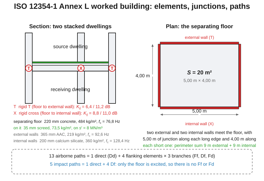
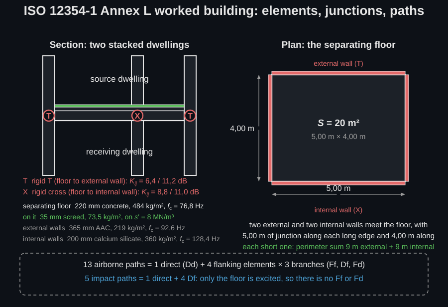
The drawing is what ties the element list to the numbers the snippet multiplies. The separating floor’s perimeter sum is 9 m of external edge plus 9 m of internal edge because the 5,00 m × 4,00 m floor meets an external wall along each 4,00 m edge and an internal wall along each 5,00 m edge, and each of those junctions carries the floor above and below it. An external wall’s own perimeter takes 8,0 m of horizontal junction (its top and bottom edges, 4,00 m each) and 2,75 m of vertical. The floor-to-external-wall junctions are rigid T, the floor-to-internal-wall junctions rigid cross. And the thirteen paths are one direct path plus three per flanking element, .
import numpy as npfrom phonometry import building
bands = np.array([50, 63, 80, 100, 125, 160, 200, 250, 315, 400, 500, 630,                  800, 1000, 1250, 1600, 2000, 2500, 3150], float)
# Annex E junctions (unrounded): floor-to-external-wall rigid T, external wall# in-line across it, floor-to-internal-wall rigid cross, internal wall in-line.k_floor_ext = building.junction_vibration_reduction("rigid_t", "corner", 484.0 / 219.0)k_ext_ext = building.junction_vibration_reduction("rigid_t", "through", 484.0 / 219.0)k_floor_int = building.junction_vibration_reduction("rigid_cross", "corner", 360.0 / 484.0)k_int_int = building.junction_vibration_reduction("rigid_cross", "through", 484.0 / 360.0)print(round(k_floor_ext, 1), round(k_ext_ext, 1))     # 6.4 11.2  (Table L.5)print(round(k_floor_int, 1), round(k_int_int, 1))     # 8.8 11.0  (Table L.6)
# The floor's perimeter: it butts into an external wall above and below at each# of its two external edges, and crosses the internal walls at the other two.a_at_ext = building.perimeter_absorption_coefficient([92.6, 92.6], [k_floor_ext] * 2)a_at_int = building.perimeter_absorption_coefficient(    [76.8, 128.4, 128.4], [building.junction_vibration_reduction(        "rigid_cross", "through", 360.0 / 484.0), k_floor_int, k_floor_int])floor_perimeter = 9.0 * (a_at_ext + a_at_int)         # 2.659 m (Formula C.4)
floor = building.HomogeneousElement("floor", 20.0, 5.0, 4.0, 484.0, 76.8, 0.005,                                    floor_perimeter, 2200.0, 3800.0)el = building.in_situ_element(floor, bands)print(np.round(el.total_loss_factor[[0, 10]], 4))     # [0.0831 0.029 ]  Table L.3print(np.round(el.sound_reduction_index[[0, 10]], 1)) # [31.8 54.9]      Table L.3print(np.round(el.impact_level[[0, 10]], 1))          # [57.3 63.6]      Table G.3print(np.round(el.absorption_length[[0, 10]], 1))     # [10.8 11.9]      Table L.4
Every printed column of Tables L.2, L.3, L.4, G.3 and G.4 comes back within 0,06 dB, and the same fixture drives both totals.
# The floating floor: 35 mm screed, m' = 73,5 kg/m2 on s' = 8 MN/m3.f0 = 160.0 * np.sqrt(8.0 / 73.5)                      # 52.8 Hz (Formula C.2)delta = building.floating_floor_improvement(bands, resonance_frequency=f0)  # 30 lg(f/f0)
wall = building.in_situ_element(building.HomogeneousElement(    "ext1", 11.0, 4.0, 2.75, 219.0, 92.6, 0.0125, 2.375, 600.0, 1900.0), bands)
# Path D1 (Df: separating floor -> external wall 1), Table L.4.d1 = building.airborne_flanking_path(    label="D1", kind="Df", element_i=el, element_j=wall,    vibration_reduction_index=k_floor_ext, coupling_length=4.0,    separating_area=20.0, delta_r_i=delta)print(np.round(d1.values[[0, 10]], 1))                # [ 41.2  93.6]  Table L.1
Assembling the direct path and all twelve flanking paths gives the apparent index per band, its energy split and the ISO 717-1 rating in one call:
# The other three flanking elements, built the way `wall` was above, each with# its own area and perimeter sum (Formula C.4); `situ` then holds all five.specs = (("ext2", 13.75, 5.0, 2.75, 219.0, 92.6, 0.0125, 2.548, 600.0, 1900.0),         ("int1", 11.0, 4.0, 2.75, 360.0, 128.4, 0.01, 1.636, 1800.0, 2500.0),         ("int2", 13.75, 5.0, 2.75, 360.0, 128.4, 0.01, 1.839, 1800.0, 2500.0))situ = {"floor": el, "ext1": wall}for spec in specs:    situ[spec[0]] = building.in_situ_element(        building.HomogeneousElement(*spec), bands)
# The twelve flanking paths, three per flanking element, each built the way# `d1` was above.paths = []for tag, name, lij in (("1", "ext1", 4.0), ("2", "ext2", 5.0),                       ("3", "int1", 4.0), ("4", "int2", 5.0)):    flank = situ[name]    cross = k_floor_ext if name.startswith("ext") else k_floor_int    through = k_ext_ext if name.startswith("ext") else k_int_int    paths += [        building.airborne_flanking_path(label=f"D{tag}", kind="Df", element_i=situ["floor"],                                        element_j=flank, vibration_reduction_index=cross,                                        coupling_length=lij, separating_area=20.0,                                        delta_r_i=delta),        building.airborne_flanking_path(label=f"{tag}d", kind="Fd", element_i=flank,                                        element_j=situ["floor"], vibration_reduction_index=cross,                                        coupling_length=lij, separating_area=20.0),        building.airborne_flanking_path(label=f"{tag}{tag}", kind="Ff", element_i=flank,                                        element_j=flank, vibration_reduction_index=through,                                        coupling_length=lij, separating_area=20.0),    ]
res = building.detailed_airborne_prediction(    bands, direct_index=building.direct_reduction_index(el.sound_reduction_index,                                                        delta_r_source=delta),    flanking_paths=paths)print(np.round(res.r_prime[[0, 10]], 1))   # [28.8 55.9]   Table L.1 totalprint(res.rating.rating, res.dominant[0])  # 57 'Dd'res.plot()                                 # per-band path-contribution bars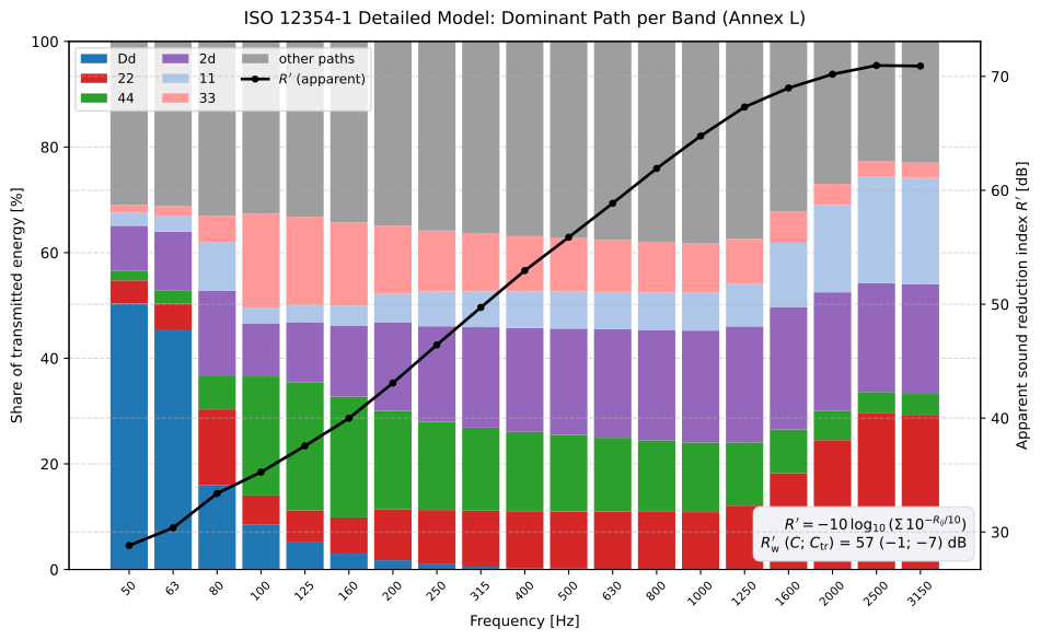
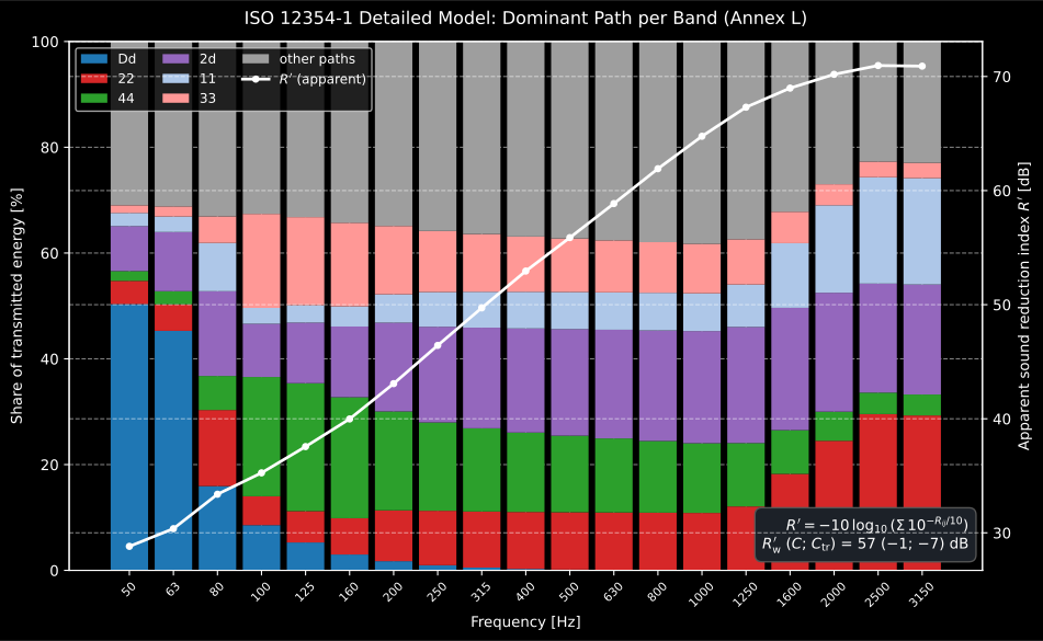
This is the plot the whole detailed model exists for. Below 80 Hz the separating floor itself is the problem, so a heavier slab or a better floating floor would help; it fades through the 80 Hz to 160 Hz transition and from 200 Hz upwards it has left the budget entirely, the flanking paths across the walls setting on their own, so no amount of work on the floor would move the result there. The single number dB says none of that.
Show the code for this figure
import matplotlib.pyplot as pltimport numpy as npfrom phonometry import building
bands = np.array([50, 63, 80, 100, 125, 160, 200, 250, 315, 400, 500, 630,                  800, 1000, 1250, 1600, 2000, 2500, 3150], float)k = {    "floor-ext": building.junction_vibration_reduction("rigid_t", "corner", 484.0 / 219.0),    "ext-ext": building.junction_vibration_reduction("rigid_t", "through", 484.0 / 219.0),    "floor-floor": building.junction_vibration_reduction("rigid_cross", "through", 360.0 / 484.0),    "floor-int": building.junction_vibration_reduction("rigid_cross", "corner", 360.0 / 484.0),    "int-int": building.junction_vibration_reduction("rigid_cross", "through", 484.0 / 360.0),    "int-ext": building.junction_vibration_reduction("rigid_t", "corner", 360.0 / 219.0),    "extT-ext": building.junction_vibration_reduction("rigid_t", "through", 360.0 / 219.0),    "corner": building.junction_vibration_reduction("corner", "corner", 1.0),    "int-int-x": building.junction_vibration_reduction("rigid_cross", "through", 1.0),}a = building.perimeter_absorption_coefficientfloor_sum = 9.0 * (a([92.6, 92.6], [k["floor-ext"]] * 2)                   + a([76.8, 128.4, 128.4],                       [k["floor-floor"], k["floor-int"], k["floor-int"]]))ext_top = a([76.8, 92.6], [k["floor-ext"], k["ext-ext"]])ext_side = a([92.6], [k["corner"]]) + a([128.4, 92.6], [k["int-ext"], k["extT-ext"]])int_top = a([76.8, 76.8, 128.4], [k["floor-int"], k["floor-int"], k["int-int"]])int_side = a([92.6, 92.6], [k["int-ext"]] * 2) + a([128.4] * 3, [k["int-int-x"]] * 3)
specs = {    "floor": (20.0, 5.0, 4.0, 484.0, 76.8, 0.005, floor_sum, 2200.0, 3800.0),    "ext1": (11.0, 4.0, 2.75, 219.0, 92.6, 0.0125,             8.0 * ext_top + 2.75 * ext_side, 600.0, 1900.0),    "ext2": (13.75, 5.0, 2.75, 219.0, 92.6, 0.0125,             10.0 * ext_top + 2.75 * ext_side, 600.0, 1900.0),    "int1": (11.0, 4.0, 2.75, 360.0, 128.4, 0.01,             8.0 * int_top + 2.75 * int_side, 1800.0, 2500.0),    "int2": (13.75, 5.0, 2.75, 360.0, 128.4, 0.01,             10.0 * int_top + 2.75 * int_side, 1800.0, 2500.0),}situ = {name: building.in_situ_element(building.HomogeneousElement(name, *spec), bands)        for name, spec in specs.items()}delta = building.floating_floor_improvement(bands,                                            resonance_frequency=160.0 * np.sqrt(8.0 / 73.5))
paths = []for tag, name, lij in (("1", "ext1", 4.0), ("2", "ext2", 5.0),                       ("3", "int1", 4.0), ("4", "int2", 5.0)):    wall = situ[name]    cross = k["floor-ext"] if name.startswith("ext") else k["floor-int"]    through = k["ext-ext"] if name.startswith("ext") else k["int-int"]    paths += [        building.airborne_flanking_path(label=f"D{tag}", kind="Df", element_i=situ["floor"],                                        element_j=wall, vibration_reduction_index=cross,                                        coupling_length=lij, separating_area=20.0,                                        delta_r_i=delta),        building.airborne_flanking_path(label=f"{tag}d", kind="Fd", element_i=wall,                                        element_j=situ["floor"], vibration_reduction_index=cross,                                        coupling_length=lij, separating_area=20.0),        building.airborne_flanking_path(label=f"{tag}{tag}", kind="Ff", element_i=wall,                                        element_j=wall, vibration_reduction_index=through,                                        coupling_length=lij, separating_area=20.0),    ]res = building.detailed_airborne_prediction(    bands,    direct_index=building.direct_reduction_index(situ["floor"].sound_reduction_index,                                                 delta_r_source=delta),    flanking_paths=paths)
# One line — the per-band path contributions with R' overlaid:res.plot()plt.show()
The impact side of the same building runs on the same situ dictionary:
from phonometry import building
k_floor_ext = building.junction_vibration_reduction("rigid_t", "corner", 484.0 / 219.0)k_floor_int = building.junction_vibration_reduction("rigid_cross", "corner", 360.0 / 484.0)direct = building.direct_impact_level(situ["floor"].impact_level, delta_l=delta)flanking = [    building.impact_flanking_path(label=f"Df{tag}", floor=situ["floor"], element_j=situ[name],                                  vibration_reduction_index=(                             k_floor_ext if name.startswith("ext") else k_floor_int),                                  coupling_length=lij, delta_l=delta)    for tag, name, lij in (("1", "ext1", 4.0), ("2", "ext2", 5.0),                           ("3", "int1", 4.0), ("4", "int2", 5.0))]imp = building.detailed_impact_prediction(bands, direct_level=direct, flanking_paths=flanking)print(np.round(imp.l_prime_n[[3, 10]], 1))     # [54.  35.9]   Table G.1 totalprint(imp.rating.rating, imp.rating.ci)        # 41 2           printed 41,0 (2)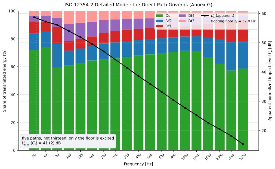
The impact half of the same building, and it is a different picture from the airborne one. There are five paths, not thirteen, because only the floor is excited: the tapping machine stands on it, so there is one direct path and one Df path into each of the four walls, and no Ff or Fd. The direct path through the excited floor governs in every band. That is the practical lesson: an impact problem is fixed at the source floor, not at the junctions.
Show the code for this figure
# One line — the per-band path contributions with L'n overlaid:imp.plot()plt.show()Read the rating the same way. dB with dB means the unweighted, walking-relevant level sits above the weighted rating, which is the signature of a floor whose improvement is concentrated high up, exactly what a floating floor with Hz and a 30 lg law does. Three levers move it, in the order the model responds to them: a softer resilient layer lowers and lifts the whole improvement curve; a heavier base slab lowers the bare level directly through Part 2’s Formula (B.2); and a better junction does almost nothing until the direct path has been dealt with. Note too that the floating floor’s is subtracted from the direct path and from every flanking path alike, because all five start at the same excited floor.
Simplified against detailed
Section titled “Simplified against detailed”The standard applies its simplified model to the same building (Tables L.10 / G.10): dB and dB against the detailed model’s dB and dB. The two agree well inside the models’ own stated spread, and the library’s test suite pins that agreement. The detailed model’s advantage is not accuracy on the single number but the spectrum behind it: the airborne prediction of the detailed model carries no bias error and a standard deviation of 1,5 dB to 2,5 dB (Clause 5) against about 2 dB for the simplified one.
Lightweight constructions (Type B)
Section titled “Lightweight constructions (Type B)”For elements whose structural reverberation time is not set by the connected elements the standard takes and describes the junction with the normalized velocity level difference instead of (Formula 17), or with a laboratory measurement of the flanking level difference (Formula 16). Below the element indices must first be corrected to resonant transmission only (Annex B.1/B.2, an 8 dB estimate for single frame elements without a cavity). The impact side offers the same two routes: Part 2 Formula (14) from and Part 2 Formula (13) from a measured normalized flanking impact level .
Unlike the Type A chain, this branch consumes measured junction data, so its
four inputs are per-band arrays over bands that come from somewhere specific.
r_wall_leaf is the leaf’s laboratory sound reduction index per band
(ISO 10140-2), corrected below its critical frequency to resonant transmission
only because a flanking path carries free bending waves alone. dv_n is the
normalized direction-averaged velocity level difference of the junction in
dB, measured per
ISO 10848-2 and referred to a
reference length of 1 m. dnf_13 is the normalized flanking level difference
of a junction measured in a laboratory, in dB, which the call re-scales
by the ratio of the site and laboratory coupling lengths. And lnf_13 is its
impact counterpart, the normalized flanking impact level in dB, which
re-scales by both area and coupling length. The block below is an excerpt: it
starts from those four arrays.
from phonometry import building
# ISO 12354-1 L.2.1: a wood frame building, floor 20 m2, junction 4 m.r_wall_leaf = ...   # measured R of the inner leaf per band, dB (ISO 10140-2)dv_n = ...          # normalized junction velocity level difference, dB (ISO 10848-2)dnf_13 = ...        # laboratory normalized flanking level difference Dn,f, dBlnf_13 = ...        # laboratory normalized flanking impact level Ln,f, dB
r_star = building.resonant_sound_reduction_index(r_wall_leaf, bands,                                                 critical_frequency=2200.0)   # +8 dB below fcr_ff = building.flanking_reduction_index_from_normalized_difference(    index_i=r_star, index_j=r_star, normalized_velocity_level_difference=dv_n,    separating_area=20.0, coupling_length=4.0)                        # Table L.11
# ISO 12354-1 L.2.2: a measured junction between two timber frame walls.r13 = building.flanking_reduction_index_from_flanking_level(    dnf_13, separating_area=10.44, coupling_length=2.41,    laboratory_coupling_length=2.5)                                   # Table L.15
# ISO 12354-2 Formula (13): the impact twin, from a measured Ln,f.ln_13 = building.flanking_impact_level_from_flanking_level(    lnf_13, area=20.0, laboratory_area=10.0,    coupling_length=4.0, laboratory_coupling_length=4.5)
Checks the standard gives you
Section titled “Checks the standard gives you”Two identities let a spectrum check itself. For a homogeneous floor the
airborne index and the impact level add up to a function of frequency alone
(Part 2 Formulae B.3/B.4), in one-third-octave bands
and in octave bands, valid where forced transmission is
negligible; reciprocity_impact_level implements it. And Table B.2 of Part 2
tabulates the octave-band of four monolithic floors calculated the way
this module does, a useful sanity target for a new floor build-up.
in_situ_element() parameters
Section titled “in_situ_element() parameters”| Parameter | Type | Units | Range / default | Notes |
|---|---|---|---|---|
element | HomogeneousElement | — | — | Area, side lengths, , , , , and optionally / |
frequencies | array | Hz | > 0 | Band centres |
bands | str | — | 'third' (default) / 'octave' | Sets the band that carries the branch |
resonant_only | bool | — | default False | Drops the forced-transmission term below (Annex B.1, flanking paths) |
fluid | Fluid | — | default EN_12354_AIR | The 340 m/s of Annex A with the 1,29 kg/m³ of Annex B; pass a computed fluids.air() to predict in the air of the building |
airborne_flanking_path() / impact_flanking_path() parameters
Section titled “airborne_flanking_path() / impact_flanking_path() parameters”| Parameter | Type | Units | Range / default | Notes |
|---|---|---|---|---|
label | str | — | — | Display name of the path |
kind | str | — | 'Ff' / 'Df' / 'Fd' | Airborne only; the impact builder is always Df |
element_i / element_j | InSituElementResult | — | — | Source-room and receiving-room elements (floor / element_j for impact) |
vibration_reduction_index | float or array | dB | — | of this path |
coupling_length | float | m | > 0 | Junction coupling length |
separating_area | float | m² | > 0 | (airborne only) |
delta_r_i / delta_r_j | float or array | dB | default 0 | Lining improvements |
delta_l | float or array | dB | default 0 | Floor-covering improvement (impact only) |
Detailed prediction report (.report())
Section titled “Detailed prediction report (.report())”DetailedAirborneResult.report() and DetailedImpactResult.report() write the
per-band counterpart of the simplified prediction fiches: the same one-page
layout, a basis line naming ISO 12354-1/-2:2017 Clause 4.2, the per-path
share-of-energy table beside the per-band path-contribution figure, the boxed
/ , the detailed model’s 1,5 dB to 2,5 dB standard deviation and a
PASS/FAIL verdict against a requirement. verbose=True annexes the band in
which each path peaks. Both need the ISO 717 rating, so the spectrum must cover
100 Hz to 3150 Hz (or 125 Hz to 2000 Hz in octaves).
res.report("airborne-prediction.pdf") # R'w, thirteen pathsimp.report("impact-prediction.pdf") # L'n,w, five pathsThe example fiches are regenerated with make reports and kept rendered in the
repository; click a preview to open the PDF. Both show the Annex L building of
this page: the same elements, junctions and floating floor the tables above are
built from.
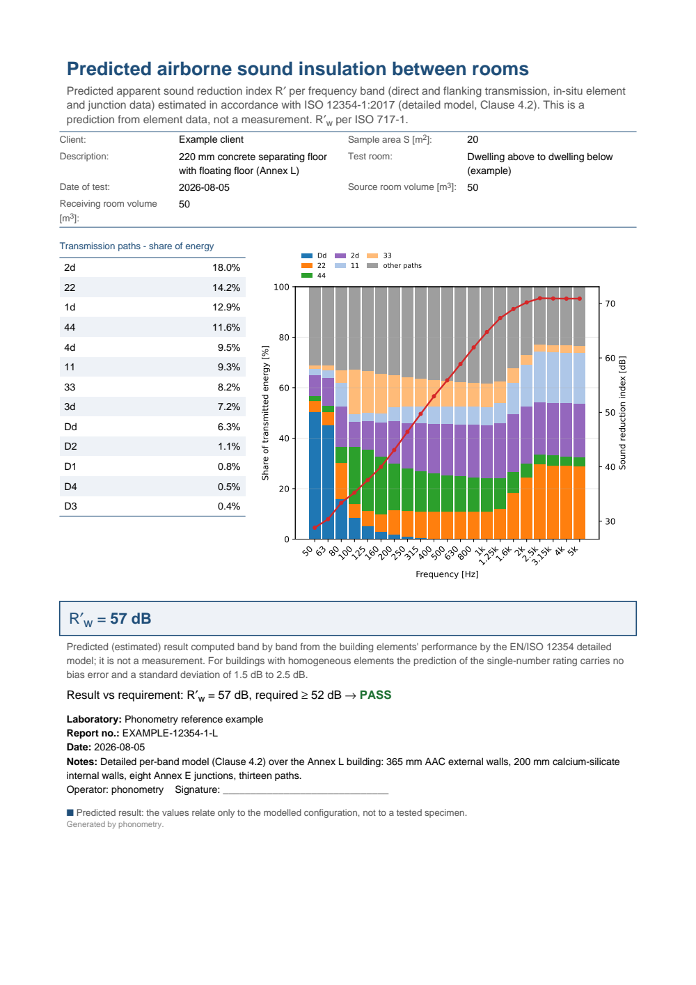
One-page detailed airborne prediction fiche for the ISO 12354-1:2017 Annex L building: an identification header with the 20 m2 separating floor and the two 50 m3 dwellings, the share-of-energy table of all thirteen paths (the 2d flanking path largest at 18.0 %, the direct Dd path 6.3 %), the per-band figure stacking each path's contribution under the apparent sound reduction index curve from 50 Hz to 5 kHz, the boxed predicted R'w = 57 dB, the detailed model's 1.5 dB to 2.5 dB standard deviation, and a PASS against a requirement of 52 dB.
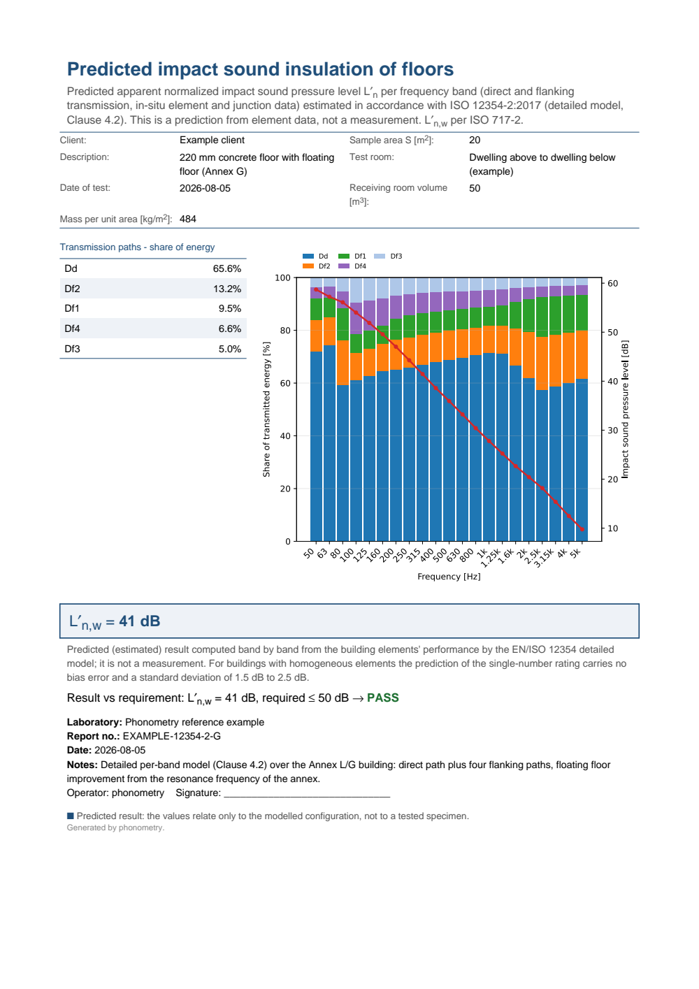
One-page detailed impact prediction fiche for the same building in the impact direction: the identification header, the share-of-energy table of the direct path and the four flanking paths, the per-band figure of each path's contribution under the apparent normalized impact sound pressure level curve, and the boxed predicted L'n,w = 41 dB with the detailed model's standard deviation and the verdict against the requirement.
What this guide covers
Section titled “What this guide covers”Covered
The Clause 4.2 per-band chain for Type A elements: the Annex B homogeneous-element sound reduction index and impact level and the Annex C in-situ conversion through
HomogeneousElement,in_situ_elementandperimeter_absorption_coefficient; the transfer of measured laboratory data throughlaboratory_total_loss_factor,structural_reverberation_time,in_situ_reduction_indexandin_situ_impact_level(Formula 9 and Part 2 Formula 5); the Formula (10) in-situ junction drop; the Formula (14)/(15) direct and flanking airborne paths throughdirect_reduction_indexandairborne_flanking_pathand their impact twinsdirect_impact_levelandimpact_flanking_path; the Formula (16)/(17) Type B routes and the Annex B.1/B.2 resonant correction throughresonant_sound_reduction_index; the assembly and ISO 717 rating throughdetailed_airborne_predictionanddetailed_impact_prediction; the Part 2 B.3/B.4 reciprocity identity throughreciprocity_impact_level; and the two fiches through.report(). The airborne model is stated by Clause 5 to carry no bias error and a standard deviation of 1,5 dB to 2,5 dB for buildings of homogeneous elements, assuming good workmanship: the lower figure when every aspect is taken into account, the higher for complex situations or when the structural reverberation time is neglected.Not covered
Only homogeneous Annex B elements are calculated here; the spectrum of a lightweight, double or composite element is an input, from Predicting Panel Sound Insulation or from a test report. The Annex E junction catalogue itself lives on Predicting Sound Insulation, and the Part 1 Annex D lining improvement on Predicting Resilient-Layer Performance; the Annex D and F default tables of EN 12354-5 are implemented nowhere. The Type B branch is shown from its standard inputs rather than worked end to end. Airborne transmission through cavities and suspended ceilings is not carried at all, and clause 3.3.4 Note 1 warns it “can contribute to or even dominate” there. And the ISO 717 rating needs the whole spectrum: 100 Hz to 3150 Hz in one-third octaves, or 125 Hz to 2000 Hz in octaves.
References
Section titled “References”- Hopkins, C. (2007). Sound insulation. Butterworth-Heinemann. https://doi.org/10.4324/9780080550473The physical background of every term of the detailed model: radiation efficiency, structural reverberation time, the equivalent absorption length and the statistical-energy-analysis footing of the path summation. ISBN 978-0-7506-6526-1.
- International Organization for Standardization. (2017). Building acoustics — Estimation of acoustic performance of buildings from the performance of elements — Part 1: Airborne sound insulation between rooms (ISO 12354-1:2017). Clause 4.2 defines the detailed per-band airborne model; Annex B the calculated element performance and radiation factors, Annex C the structural reverberation time, Annex E the junction indices and Annex L the worked examples.
- International Organization for Standardization. (2017). Building acoustics — Estimation of acoustic performance of buildings from the performance of elements — Part 2: Impact sound insulation between rooms (ISO 12354-2:2017). Clause 4.2 defines the detailed per-band impact model; Annex B the calculated impact level of a bare floor, Annex C the floating-floor improvement and Annex G the worked examples sharing ISO 12354-1 Annex L's building.
- Vigran, T. E. (2008). Building acoustics. Taylor & Francis. The homogeneous-element transmission model and the impact-level closed form behind Annex B of both parts. ISBN 978-0-415-42853-8.