Laboratory Flanking Transmission (ISO 10848)

EN 12354 predicts a building from its junctions, and ISO 10848 is how a junction gets its number. Two elements rigidly joined along a common edge are built into a laboratory rig whose rooms are structurally isolated from each other and from the surrounding structure, so the junction under test is the only path between them; shakers and tapping machines drive one element, and the velocity level differences across the junction condense into the vibration reduction index $K_{ij}$, together with the overall flanking descriptors $D_{n,f}$ (airborne) and $L_{n,f}$ (impact). This guide covers that measurement chain: the direction-averaged velocity level difference, the equivalent absorption lengths, the SEA validity checks of Part 4 and the three accredited-report-style fiches. The empirical junction values a prediction falls back on when no measurement exists live in Predicting Sound Insulation (EN 12354); the wave-theory $K_{ij}$ of ideal plate junctions is derived in Bending-wave transmission at plate junctions.

The vibration reduction index and the flanking descriptors

ISO 10848:2006/2010 is the laboratory method that measures the junction vibration reduction index $K_{ij}$ that the EN 12354 prediction takes as an input, together with the overall flanking descriptors $D_{n,f}$ (airborne) and $L_{n,f}$ (impact). It is the measurement counterpart of the empirical junction_vibration_reduction() of that prediction.

Vibration reduction index (Formula (13)). $K_{ij}={\overline{D}}_{v,ij}+10{\log }_{10}(l_{ij}/\sqrt{a_i{a}_j})$ dB, from the direction-averaged velocity level difference ${\overline{D}}_{v,ij}=\frac{1}{2}(D_{v,ij}+D_{v,ji})$ (Formula (11), which makes $K_{ij}$ symmetric), the common-edge junction length $l_{ij}$ and the equivalent absorption lengths $a_j=2.2{\pi }^2{S}_j/(T_{s,j}{c}_0)\sqrt{f_{\text{ref}}/f}$ (Formula (12), $f_{\text{ref}}=1000$ Hz). For lightweight well-damped elements $a_j=S_j/l_0$ ($l_0=1$ m) and Formula (13) reduces to the simplified Formula (14), which needs no $T_s$ at all.

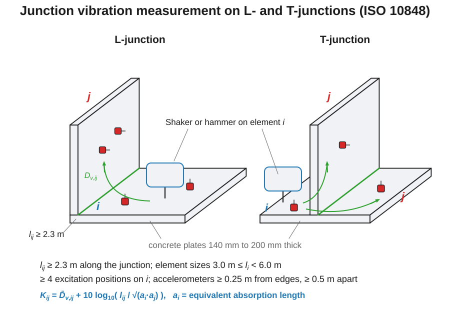
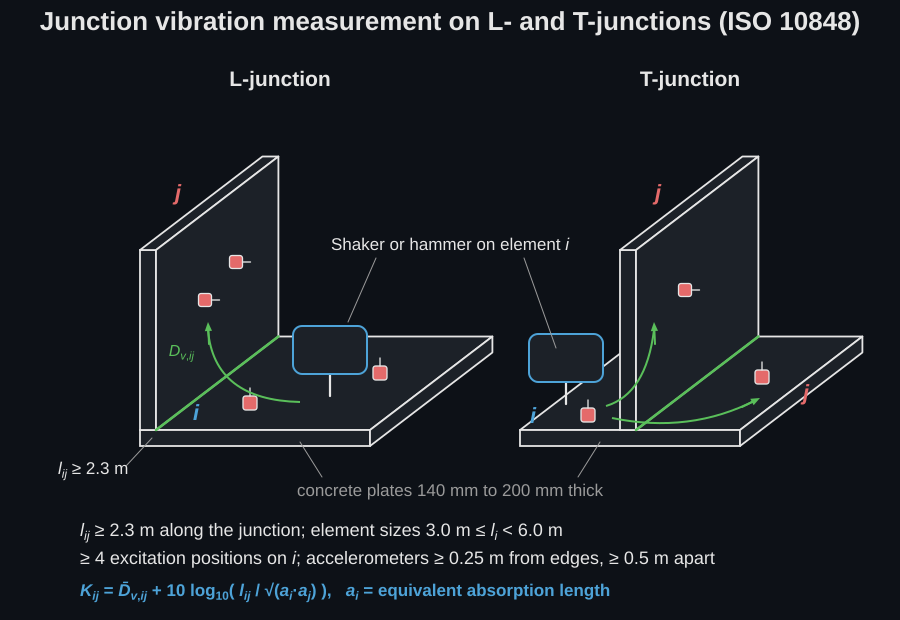
Every symbol in Formula (13) is a length or an area in that drawing. The highlighted corner line is $l_{ij}$, the common edge of the two elements; $S_i$ and $S_j$ are the areas of the two plates, which enter through their equivalent absorption lengths $a_i$ and $a_j$; and ${\overline{D}}_{v,ij}$ is what the pair of accelerometers reads, once with element $i$ driven and once with element $j$ driven. The $10{\log }_{10}(l_{ij}/\sqrt{a_i{a}_j})$ term is what makes the index a property of the junction rather than of the two particular plates that were built into the rig, which is the entire reason EN 12354 can consume it.

The structural reverberation time, and where it comes from

$T_{s,j}$ is the second most influential input on this page and the one most often assumed. It is not the room’s reverberation time: it is the decay of bending-wave energy on the element itself, measured with accelerometers, and it is what carries the element’s total loss factor into the absorption length, ${\eta }_{\text{total}}=2.2/(f{T}_s)$ (ISO 10848-1:2017, Formula (19)). Because $a_j\propto 1/T_{s,j}$ and $K_{ij}$ carries $-10{\log }_{10}\sqrt{a_i{a}_j}$, a $T_s$ wrong by a factor of two moves $K_{ij}$ by 1.5 dB in each element, and it moves it in the direction that makes a junction look better than it is when $T_s$ is overestimated.

Measure it as ISO 10848-1:2017 Clause 7.3 prescribes: point excitation by an electrodynamic shaker with an MLS or swept-sine signal (the preferred laboratory method, per ISO 18233) or by an impact hammer, the integrated impulse response of ISO 3382-2 with backward integration, acceleration rather than velocity so no integration smears the decay, at least three excitation positions and three measurement positions per excitation, and the minimum separations of Clause 7.3.3 (0.5 m from the element boundaries, 1 m between the excitation and the measurement positions, 0.5 m between measurement positions). Evaluate over 5 dB to 15 dB from a decay that starts at least 35 dB above the background (Clause 7.3.4); heavy elements coupled to other heavy elements give a short straight decay followed by a curve as energy returns from the rest of the structure, so the short evaluation range is not a convenience but a requirement of the physics. Clause 7.3.5 sets the floor below which a forward analysis stops being reliable: $T_s>70/f$ and $T_s>2T_{\text{det}}$, with $T_{\text{det}}$ the reverberation time of the averaging detector.

Expect a few tenths of a second on a heavy concrete plate built into a building, falling with frequency, and much less on a well-damped lightweight element — which is why the lightweight route of Formula (14) drops $T_s$ entirely. The loss-factor identity is the sanity check on a measured value: at 500 Hz a $T_s$ of 0.35 s gives $\eta =2.2/(500\times 0.35)=0.013$, a plausible total loss factor for an in-situ heavy plate, while an $\eta$ coming out above about 0.1 or below 0.005 says the decay was misread rather than that the plate is unusual.

Overall descriptors. $D_{n,f}=L_1-L_2-10{\log }_{10}(A/A_0)$ (Formula (4), airborne) and $L_{n,f}=L_2+10{\log }_{10}(A/A_0)$ (Formula (5), tapping machine), $A_0=10{\text{m}}^2$; their $D_{n,f,w}$ / $L_{n,f,w}$ single numbers reuse the ISO 717 rating engines. The single-number ${\overline{K}}_{ij}$ is the arithmetic mean over 200–1250 Hz for one-third-octave bands, or over 125–1000 Hz for octave bands (Annex A).

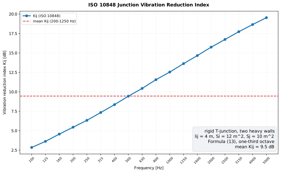
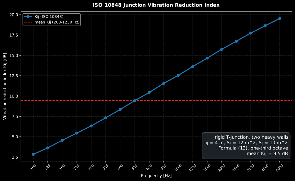
$K_{ij}$ climbs steadily with frequency for a rigid junction of heavy walls, so no single band represents it. The dashed line is the arithmetic mean over 200–1250 Hz, the range Annex A prescribes, and it is that mean — not the curve — that an EN 12354 prediction consumes.

Show the code for this figure

import matplotlib.pyplot as plt
import numpy as np
from phonometry import building

freqs = [100, 125, 160, 200, 250, 315, 400, 500, 630,
         800, 1000, 1250, 1600, 2000, 2500, 3150, 4000, 5000]
# Direction-averaged velocity level difference of a rigid T-junction (dB):
dv = np.array([4.5, 4.8, 5.2, 5.6, 6.0, 6.5, 7.0, 7.6, 8.1, 8.7,
               9.2, 9.8, 10.3, 10.9, 11.4, 11.9, 12.3, 12.7])
res = building.vibration_reduction_index(
    dv, junction_length=4.0, area_i=12.0, area_j=10.0, frequency=freqs,
    structural_reverberation_time_i=0.35, structural_reverberation_time_j=0.40,
)
print(res.single_number)   # mean Kij over 200-1250 Hz (Annex A)
res.plot()
plt.show()

Validity. $K_{ij}$ rests on a statistical-energy-analysis simplification: strong_coupling_satisfied() checks the Formula (15) inequality and, for the heavy junctions of Part 4, modal_density(), band_mode_count() and modal_overlap_factor() (Formulae (5)/(4)/(6)) quantify where the mode count is too low for $K_{ij}$ to be reliable. Pass the per-band modal overlap factor to vibration_reduction_index(..., modal_overlap=M): bands with $M<0.25$ are flagged in result.bracketed and excluded from the single-number ${\overline{K}}_{ij}$, as Part 4 Clause 9 requires. Because ISO 10848 contains no worked numeric example, conformance is anchored on closed-form identities (simplified $K_{ij}$, $a_j$ at $f_{\text{ref}}$, $\eta$).

import numpy as np
from phonometry import building

freqs = [200, 250, 315, 400, 500, 630, 800, 1000, 1250]
lij, s_i, s_j = 4.0, 12.0, 10.0     # junction length (m), element areas (m^2)
ts = np.linspace(0.30, 0.10, 9)     # structural reverberation time Ts (s)
dv_ij = [5.6, 6.0, 6.5, 7.0, 7.6, 8.1, 8.7, 9.2, 9.8]    # element i excited (dB)
dv_ji = [6.4, 6.8, 7.3, 7.8, 8.4, 8.9, 9.5, 10.0, 10.6]  # element j excited (dB)

# Kij from both excitation directions (symmetric via the direction average):
dbar = building.direction_averaged_level_difference(dv_ij, dv_ji)
res = building.vibration_reduction_index(dbar, lij, s_i, s_j, frequency=freqs,
                                structural_reverberation_time_i=ts,
                                structural_reverberation_time_j=ts)
res.k_ij           # Kij per band (Formula (13))
res.single_number  # mean Kij over 200-1250 Hz, or None without the band set
res.octave_bands() # Kij in octave bands (its single number averages 125-1000 Hz)

# Overall airborne flanking descriptor and a Part-4 modal-overlap validity check:
dnf = building.normalized_flanking_level_difference(np.full(9, 75.0), np.full(9, 42.0),
                                           absorption_area=np.full(9, 12.0))
m = building.modal_overlap_factor(s_i, critical_frequency=85.0,
                         structural_reverberation_time=ts)
res_m = building.vibration_reduction_index(dbar, lij, s_i, s_j, frequency=freqs,
                                  modal_overlap=m)   # M < 0.25 bands bracketed
res_m.bracketed    # per-band flags; bracketed bands leave the single number

# With 16 one-third-octave (or 5 octave) bands, dnf.plot() draws Dn,f vs the
# shifted ISO 717-1 reference with Dn,f,w annotated (needs matplotlib):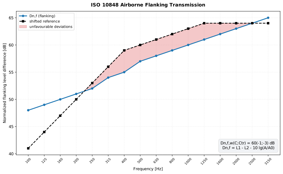

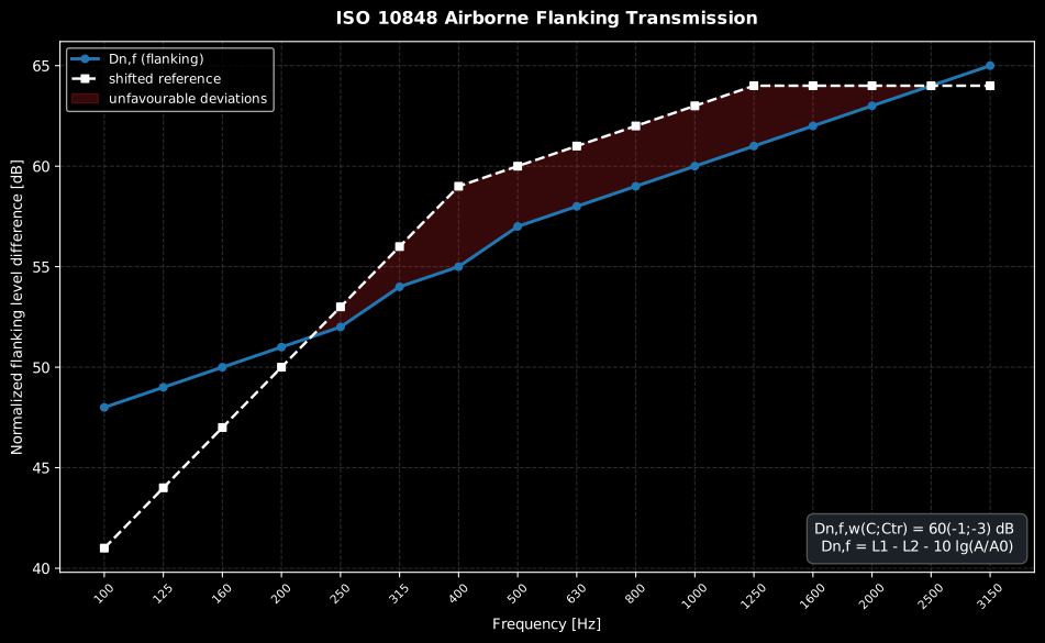
The overall flanking descriptor $D_{n,f}$ is an airborne quantity, so its single number $D_{n,f,w}$ comes from the unchanged ISO 717-1 engine; it drops straight into the EN 12354-1 model as the flanking-path datum of the tested junction (the impact counterpart $L_{n,f}$ rates per ISO 717-2 the same way).

Show the code for this figure

import matplotlib.pyplot as plt
import numpy as np
from phonometry import building

# A lightweight junction in the laboratory: source-room level, receiving-room
# level over the flanking path, and the receiving-room absorption area.
l1 = np.full(16, 80.0)
dnf_target = np.array([48, 49, 50, 51, 52, 54, 55, 57,
                       58, 59, 60, 61, 62, 63, 64, 65], dtype=float)
dnf = building.normalized_flanking_level_difference(
    l1, l1 - dnf_target, absorption_area=np.full(16, 10.0)
)

# One line — Dn,f vs the shifted ISO 717-1 reference:
dnf.plot()
plt.show()

# By hand, from the rating the result carries:
w = dnf.rating
fig, ax = plt.subplots()
ax.semilogx(w.band_centers, dnf.d_n_f, "o-", label="Dn,f (flanking)")
ax.semilogx(w.band_centers, w.shifted_reference, "s--",
            label="shifted reference")
ax.fill_between(w.band_centers, w.measured, w.shifted_reference,
                where=w.measured < w.shifted_reference, interpolate=True,
                alpha=0.3, label="unfavourable deviations")
ax.set_xlabel("Frequency [Hz]")
ax.set_ylabel("Normalized flanking level difference [dB]")
ax.set_title(f"Dn,f,w = {w.rating} dB  (C={w.c:+d}; Ctr={w.ctr:+d})")
ax.legend()
plt.show()

Making the measurement (ISO 10848-1:2017, Clauses 7 and 9)

The formulae above are indifferent to how their inputs were obtained. The standard is not, and one of its requirements decides whether the number means anything at all.

Shielding comes first (Clause 9). A junction of three or four elements has two elements facing each room, and a receiving-room level fed by all of them is not attributable to any one path. So the elements not under test are shielded, successively, and the rule differs by quantity: measuring $D_{n,f}$ for transmission through $i$ and $j$, shield the other element in both rooms; measuring $L_{n,f}$, shield the other element in the receiving room; measuring $K_{ij}$ with structure-borne excitation, no shielding is needed, because the excitation is applied to one element rather than to a sound field. Radiated sound measured by intensity to ISO 15186-1 also needs no receiving-room shielding, because the enclosing surface does the same job.

The shield has to be good enough to be worth building. Where the three or four elements of the junction are identical, a $\Delta R$ of 10 dB in every band suffices. In general, excite element 1 and then element 2 with the same kind of excitation, read the average velocity level of the receiving element $j$ in each case, and require $\Delta R_{\text{min}}=10-L_{v,1j}+L_{v,2j}$ when $L_{v,1j}-L_{v,2j}\le 10$ dB, and nothing at all when the difference already exceeds 10 dB (Formulae (23) and (24)). Heavy shielding on a light element can change the very transmission being measured and is to be avoided. A $K_{ij}$ or $D_{n,f}$ quoted without a statement of how the other elements were shielded, and of how that shielding was verified, is a room-pair number with a path label attached to it — and it flows straight into an EN 12354 prediction, where the error is unbounded in direction.

Accelerometers (Clause 7.2.3). Mounted directly on the surface of the test element, stiff in the direction normal to it. Bees or petroleum wax is convenient, but a weak fixing costs high-frequency accuracy; where the surface texture defeats wax, cement a small metal washer to it and wax or stud onto that (ISO 5348). The accelerometer mass must be small enough not to load the plate, which Formula (16) makes explicit: $m_{\text{acc}}<1/(2\pi f{Y}_{\text{dp}})$, with the driving-point mobility of a thin isotropic plate estimated by Formula (17) as $Y_{\text{dp}}=1/(8\sqrt{B{\rho }_s})=1/(2.3{\rho }_s{c}_{L}h)$. The inequality bites at the top of the band range, so check it at the highest band, not the lowest.

Excitation (Clause 7.2.4). Steady-state, from an electrodynamic shaker driven with noise or from a tapping machine (adapted for walls, with the impacts mechanically controlled to repeat), or transient, from single or manually repeated hammer blows — in which case $D_{v,ij}$ must be measured on both elements simultaneously. Manual multiple hits are spread over 1 m² to 2 m² at 1 Hz to 2 Hz over 20 s to 30 s. In every band the receiving element’s velocity level must exceed the background by at least 10 dB; below that, the ISO 10140-4 correction applies and must not exceed 1.3 dB. Take care that the source’s own airborne noise, or radiation from the excited element, does not excite the others — that is the same failure the shielding exists to prevent, arriving by a different route.

Positions (Clause 7.2.5). At least four excitation positions on a Type A (heavy, homogeneous) source element and six on a Type B one, with at least three measurement positions per excitation position on each plate, randomly distributed over the surface rather than gridded. The minimum separations are: 0.5 m from an excitation position to the element boundaries, 1.0 m between excitation positions (0.7 m for Type B), 1.0 m from an excitation position to the junction under test, 1.0 m from an excitation position to its associated measurement positions, 0.25 m from a measurement position to the element boundaries and 0.5 m between the measurement positions of one excitation position. On inhomogeneous elements (hollow brick, beam-and-block) the positions must also be spread over the sub-elements, and on framed floors the tapping-machine axis sits at 45° to the joists. On lightweight junctions the operator should stay off the floor unless their weight and damping can be shown not to matter.

Both directions. $K_{ij}$ is symmetric only because the standard makes it so: run the whole procedure with element $i$ excited and again with element $j$ excited, and average the two level differences before Formula (13), which is exactly what direction_averaged_level_difference does in the snippet above.

Suspended ceilings: the plenum flanking path (ISO 140-9, Vigran 9.2.3)

Two offices separated by a partition that stops at the suspended ceiling share one continuous plenum above it. Sound leaves the source room through the ceiling tiles, travels sideways over the partition and comes back down through the tiles of the receiving room. That path is often the weakest link in an open-plan fit-out, and it is not what a partition’s $R_w$ describes.

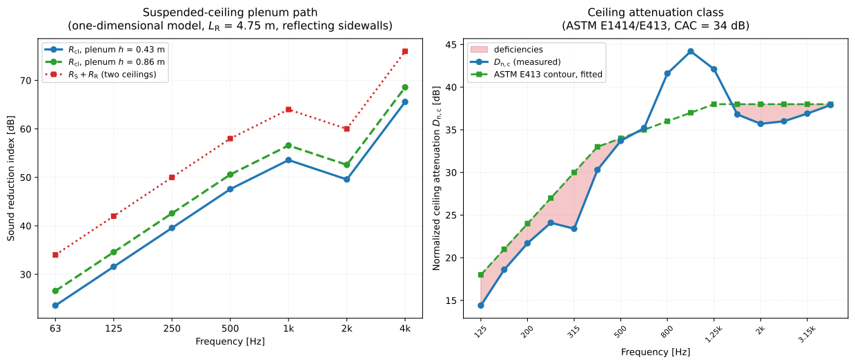
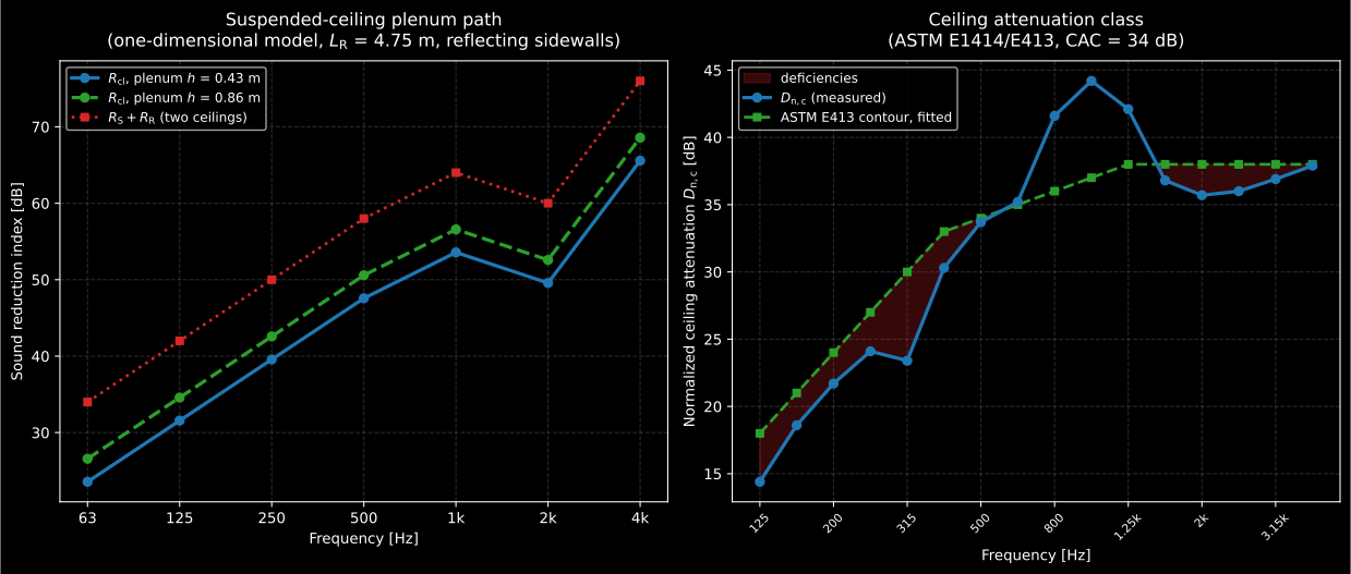
Left: the plenum charges a fixed penalty against the sum of the two ceilings — about 10 dB for this geometry — and doubling its depth pays back only 3 dB of it, which is why the tile is the lever and the void is not. Right: the same quantity as an accredited laboratory measures it, with the ASTM E413 contour fitted to the measured $D_{n,c}$ and its deficiencies shaded; the class is read off the shifted contour at 500 Hz.

Show the code for this figure

import matplotlib.pyplot as plt
import numpy as np

from phonometry import ceiling_attenuation_class, plenum_flanking_reduction_index

fig, (ax_path, ax_cac) = plt.subplots(1, 2, figsize=(13.0, 5.6))

# Left: Vigran Section 9.2.3 geometry, LS = LR = 4.75 m, 9.5 mm plasterboard
# ceiling, reflecting plenum sidewalls, at two plenum depths.
freqs = np.array([63.0, 125.0, 250.0, 500.0, 1000.0, 2000.0, 4000.0])
ceiling = np.array([17.0, 21.0, 25.0, 29.0, 32.0, 30.0, 38.0])
x = np.arange(freqs.size)
for depth, style in ((0.43, "-o"), (0.86, "--o")):
    res = plenum_flanking_reduction_index(
        ceiling, ceiling, ceiling_length=4.75, plenum_height=depth,
        frequency=freqs,
    )
    ax_path.plot(x, res.reduction_index, style, label=f"Rcl, plenum h = {depth:g} m")
ax_path.plot(x, 2.0 * ceiling, ":s", label="RS + RR (two ceilings)")
ax_path.set_xticks(x, ["63", "125", "250", "500", "1k", "2k", "4k"])
ax_path.set(xlabel="Frequency [Hz]", ylabel="Sound reduction index [dB]")
ax_path.legend()

# Right: an accredited ASTM E1414 test report rated per ASTM E413.
dnc = np.array([14.4, 18.6, 21.7, 24.1, 23.4, 30.3, 33.7, 35.2,
                41.6, 44.2, 42.1, 36.8, 35.7, 36.0, 36.9, 37.9])
cac = ceiling_attenuation_class(dnc)
xc = np.arange(dnc.size)
ax_cac.fill_between(xc, cac.measured, cac.shifted_reference,
                    where=cac.measured < cac.shifted_reference,
                    interpolate=True, alpha=0.25, label="deficiencies")
ax_cac.plot(xc, cac.measured, "-o", label="Dn,c (measured)")
ax_cac.plot(xc, cac.shifted_reference, "--s", label="ASTM E413 contour, fitted")
ax_cac.set(xlabel="Frequency [Hz]",
           ylabel="Normalized ceiling attenuation Dn,c [dB]",
           title=f"CAC = {cac.rating} dB")
ax_cac.legend()
plt.show()

The one-dimensional model

Mechel’s one-dimensional variant, as presented by Vigran in Section 9.2.3, treats the plenum as a duct lined on one side. The ceiling on each side has a transmission factor ${\tau }_S={\tau }_{S,pl}{\tau }_{S,a}$ (plates times any plenum absorber, Eq. (9.14)); the injected power splits, a fraction $s_S$ heading for the partition, and decays as $\exp (-mx)$ with the power attenuation coefficient $m=2\mathrm{Re}\{\Gamma \}=-2\mathrm{Im}\{k^{\prime }\}$ (Eqs. (9.15) and (9.16)). Integrating over the ceiling length on both sides gives Eq. (9.18), whose receiving side carries the leakage back into the room, $m_R^{\prime }=m_R+s_R{\tau }_R/h$ (Eq. (9.17)). Vigran prints the unprimed $m_R$ in that expression’s denominator; that is a misprint, recorded in the errata register, and the derived $m_R^{\prime }$ is used here. Read literally, the printed form is non-monotonic in the plenum damping (adding absorber would predict a worse path than none) and unbounded as $m_R\to 0$. For a plenum with little attenuation and $s_S=s_R=0,5$ that collapses to the compact form that makes the geometry visible (Eqs. (9.19) and (9.20)):

$$R_{cl}=R_S+R_R-10{\log }_{10}\left[\frac{{\epsilon }^2{L}_R}{4h}\right],$$

with $\epsilon =1$ for totally absorbing plenum sidewalls and $\epsilon =2$ for totally reflecting ones. A deep plenum helps, a long room hurts, and doubling the tile insulation helps twice over because $R_S$ and $R_R$ both appear. Referred to the partition area instead of the ceiling, $R_{cl,p}=R_{cl}+10{\log }_{10}(H_S/L_S)$ (Eq. (9.13)), which is what lets the ceiling path be added to the direct path as transmission factors.

from phonometry import partition_referenced_reduction_index
# `plenum_flanking_reduction_index` is the import of the figure block above.

freqs = [63.0, 125.0, 250.0, 500.0, 1000.0, 2000.0, 4000.0]
ceiling = [17.0, 21.0, 25.0, 29.0, 32.0, 30.0, 38.0]   # 9.5 mm plasterboard

# Vigran's example geometry: LS = LR = 4.75 m, plenum 0.43 m, reflecting walls.
res = plenum_flanking_reduction_index(
    ceiling, ceiling, ceiling_length=4.75, plenum_height=0.43, frequency=freqs
)
print(round(res.geometry_term, 1))    # 10.4 dB charged against RS + RR
res.plot()                            # Rcl against the two ceilings

# A lined plenum attenuates the sideways path (Eq. (9.18) instead of (9.20)):
damped = plenum_flanking_reduction_index(
    ceiling, ceiling, ceiling_length=4.75, plenum_height=0.43,
    attenuation_source=[0.5] * 7, attenuation_receiving=[0.5] * 7,
)

# Referred to the partition instead of the ceiling (Eq. (9.13)):
print(partition_referenced_reduction_index(res.reduction_index, 2.7, 4.75))

The measured quantity: normalized ceiling attenuation

A ceiling is not rated by $R_{cl}$ but by the normalized ceiling attenuation $D_{n,c}=D-10{\log }_{10}(A/A_0)$ (ISO 140-9:1985 clause 3.3), with $A$ the receiving-room equivalent absorption area and the reference $A_0=10{\text{m}}^2$. The facility has two rooms of at least 50 m³ whose volumes differ by at least 10 %, a dividing wall tapered to at most 100 mm at the top, and a plenum 650 mm to 760 mm deep with one sidewall and both end walls lined; the standard prints the required lining absorption ${\alpha }_s\ge 0,65$ at 125 Hz and $\ge 0,80$ from 250 Hz to 4000 Hz, and requires $\alpha <0,10$ on the other sidewall and on the plenum ceiling. The North American counterpart, ASTM E1414, uses $A_0=12{\text{m}}^2$, so an ASTM value runs about $10{\log }_{10}(12/10)=0,79$ dB higher for the same rooms.

ISO rates $D_{n,c}$ with the ISO 717-1 curve, giving $D_{n,c,w}$; ASTM E1414 rates it through ASTM E413 as the ceiling attenuation class. E413 rounds the data to the nearest integer (clause 5.2), raises its reference contour in 1 dB steps while the sum of the deficiencies stays at or below 32 dB and no single deficiency exceeds 8 dB (clauses 5.3 and 5.4), and reads the rating off the shifted contour at 500 Hz (clause 5.5).

from phonometry import normalized_ceiling_attenuation, weighted_rating
# `ceiling_attenuation_class` is the import of the figure block above.

# Dn,c from the measured pair: source- and receiving-room levels over the
# common plenum and the receiving room's absorption area, per band. ASTM E1414
# normalizes to A0 = 12 m2, ISO 140-9 to A0 = 10 m2.
l1_c = [80.0] * 16                       # source room, per band
l2_c = [45.0] * 16                       # receiving room, over the plenum path
absorption = [12.0] * 16                 # receiving-room A per band (m2)
astm = normalized_ceiling_attenuation(l1_c, l2_c, absorption, reference_area=12.0)
iso140_9 = normalized_ceiling_attenuation(l1_c, l2_c, absorption)
print(round(float(astm[0]), 2), round(float(iso140_9[0]), 2))   # 35.0 34.21

# A 28 mm perforated plaster acoustic tile, measured to ASTM E1414 (CAC 34).
dnc = [14.4, 18.6, 21.7, 24.1, 23.4, 30.3, 33.7, 35.2,
       41.6, 44.2, 42.1, 36.8, 35.7, 36.0, 36.9, 37.9]
res = ceiling_attenuation_class(dnc)
print(res.rating, res.deficiency_sum, res.max_deficiency)   # 34, 27.0, 7.0
res.plot()                                                  # Dn,c vs the contour

# The ISO single number of the same spectrum, shifted to A0 = 10 m2:
iso = [v - 0.79 for v in dnc]
print(weighted_rating(iso).rating)                          # Dn,c,w

ISO 10848 flanking-transmission reports (.report())

Each of the three results renders a one-page PDF fiche. VibrationReductionResult.report() writes a junction characterization report of $K_{ij}$ (ISO 10848-1:2006): the standard-basis line, an optional metadata header, the per-band $K_{ij}$ table beside the $K_{ij}(f)$ curve and a boxed single-number mean $K_{ij}$ over the Annex A band range, with the count of averaged and bracketed bands. Bands bracketed for poor modal overlap ($M<0.25$, ISO 10848-4:2010 Clause 9) print their value in brackets and are excluded from the mean; verbose=True adds a column stating whether each band enters the mean.

FlankingLevelDifferenceResult.report() and FlankingImpactLevelResult.report() write measurement reports of the overall descriptors $D_{n,f}$ (airborne) and $L_{n,f}$ (impact, tapping machine), reusing the same two-panel insulation layout: the per-band quantity beside the measured-versus-shifted-ISO 717-reference curve and the boxed single number $D_{n,f,w}$ (C; Ctr) (ISO 717-1) or $L_{n,f,w}$ (CI) (ISO 717-2). verbose=True annexes the ISO 717 evaluation per band (the value, the shifted reference and the unfavourable deviation). A requirement supplied on the ReportMetadata adds a verdict ($D_{n,f,w}$ passes at or above it, $L_{n,f,w}$ at or below it), and language="es" renders every fiche in Spanish. reportlab is required, and matplotlib too for the figure the fiche embeds (pip install "phonometry[report,plot]").

import numpy as np
from phonometry import building, ReportMetadata

freqs = [100, 125, 160, 200, 250, 315, 400, 500, 630,
         800, 1000, 1250, 1600, 2000, 2500, 3150, 4000, 5000]
dv = np.array([4.5, 4.8, 5.2, 5.6, 6.0, 6.5, 7.0, 7.6, 8.1, 8.7,
               9.2, 9.8, 10.3, 10.9, 11.4, 11.9, 12.3, 12.7])
m = np.full(18, 1.0); m[:3] = 0.1                        # bracket the low bands
kij = building.vibration_reduction_index(
    dv, junction_length=4.0, area_i=12.0, area_j=10.0, frequency=freqs,
    structural_reverberation_time_i=0.35, structural_reverberation_time_j=0.40,
    modal_overlap=m,
)
kij.report("Kij.pdf", metadata=ReportMetadata(specimen="Rigid T-junction"))

l1 = np.full(16, 80.0)
dnf = np.array([48, 49, 50, 51, 52, 54, 55, 57, 58, 59, 60, 61, 62, 63, 64, 65],
               dtype=float)
dres = building.normalized_flanking_level_difference(
    l1, l1 - dnf, absorption_area=np.full(16, 10.0)
)
dres.report("Dnf.pdf", metadata=ReportMetadata(requirement=55.0))   # Dn,f,w (C; Ctr)

recv = np.array([58, 57, 56, 55, 54, 52, 50, 48, 46, 44, 42, 40, 38, 36, 34, 32],
                dtype=float)
lres = building.normalized_flanking_impact_level(recv, absorption_area=np.full(16, 10.0))
lres.report("Lnf.pdf", metadata=ReportMetadata(requirement=55.0))   # Ln,f,w (CI)

The example fiches are regenerated with make reports and kept in the repository. Click a preview to open the PDF:

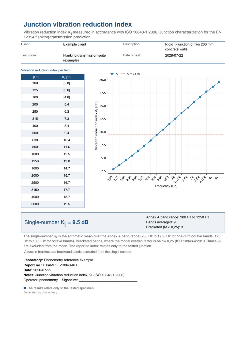
One-page junction-characterization report of the vibration reduction index Kij: the metadata header, the per-band Kij table beside the Kij(f) curve, and the boxed single-number mean Kij over the Annex A band range with the count of averaged and bracketed bands (the three lowest bands bracketed for poor modal overlap).

Download the report (PDF)

Vibration reduction index fiche (VibrationReductionResult.report), mean Kij.

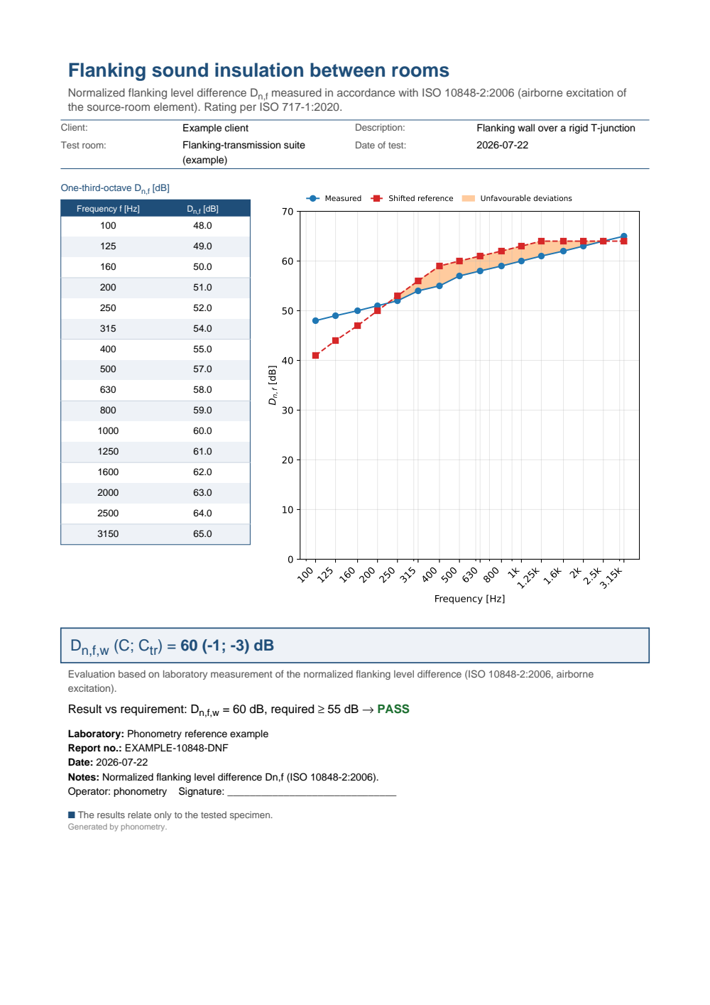
One-page airborne flanking-transmission report of the normalized flanking level difference Dn,f: the metadata header, the one-third-octave Dn,f table beside the measured-versus-shifted-reference curve, the boxed Dn,f,w (C; Ctr) rated per ISO 717-1 and a PASS verdict against the 55 dB requirement.

Download the report (PDF)

Flanking level difference fiche (FlankingLevelDifferenceResult.report), Dn,f,w (C; Ctr).

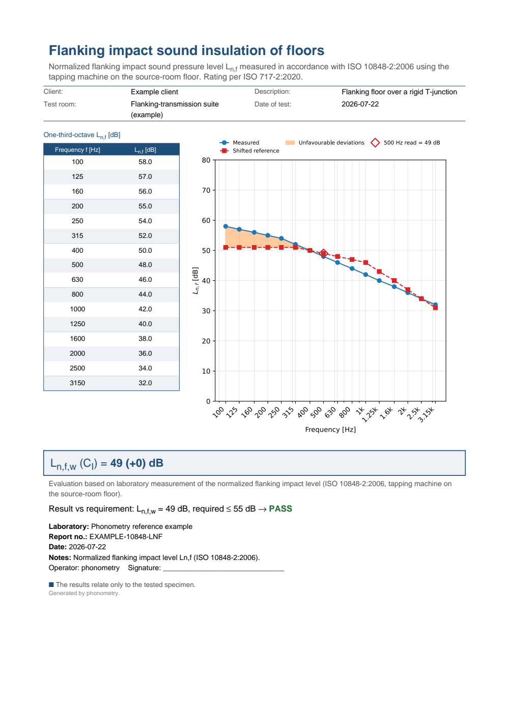
One-page impact flanking-transmission report of the normalized flanking impact level Ln,f: the metadata header, the one-third-octave Ln,f table beside the measured-versus-shifted-reference curve, the boxed Ln,f,w (CI) rated per ISO 717-2 and a PASS verdict against the 55 dB requirement.

Download the report (PDF)

Flanking impact level fiche (FlankingImpactLevelResult.report), Ln,f,w (CI).

What this guide covers

• Covered

  ISO 10848-1:2006’s vibration reduction index $K_{ij}$ (Formula (13)) from the direction-averaged velocity level difference (Formula (11)) and the equivalent absorption lengths (Formula (12)), with the simplified lightweight form (Formula (14)), the total loss factor and the Annex A single-number mean, via building.direction_averaged_level_difference and building.vibration_reduction_index; the overall descriptors $D_{n,f}$ (Formula (4)) and $L_{n,f}$ (Formula (5)) with their ISO 717 single numbers, via building.normalized_flanking_level_difference and building.normalized_flanking_impact_level; the strong-coupling check (Formula (15)) and the ISO 10848-4:2010 modal-density, band-mode-count and modal-overlap validity checks that bracket unreliable bands (building.strong_coupling_satisfied, building.modal_density, building.band_mode_count, building.modal_overlap_factor); and the three one-page fiches through .report().

• Not covered

  ISO 10848 Parts 2, 3 and 4 differ in which junction and specimen types they apply to; phonometry implements only the Part 1 $K_{ij}$/$D_{n,f}$/$L_{n,f}$ formulae generically, plus the Part 4 modal-overlap validity check, not the facility-specific test setups the other parts describe. The acquisition of Making the measurement is documented here and enforced nowhere: nothing checks that the other elements were shielded, that the shield met $\Delta R_{\text{min}}$, that the position counts and separations were kept, that the accelerometer satisfied the mass-loading inequality, or that $T_s$ was measured on the elements in their installed state rather than assumed. Because ISO 10848 contains no worked numeric example, conformance is anchored on closed-form identities (simplified $K_{ij}$, $a_j$ at $f_{\text{ref}}$, $\eta$).

• Covered

  The suspended-ceiling branch covers the normalized ceiling attenuation $D_{n,c}$ of ISO 140-9:1985 clause 3.3, the ASTM E413-22 ceiling attenuation class that ASTM E1414 invokes, and the one-dimensional plenum model of Vigran Section 9.2.3, via building.normalized_ceiling_attenuation, building.ceiling_attenuation_class, building.plenum_flanking_reduction_index and building.partition_referenced_reduction_index. The plenum model has no published numeric output of its own, so it is anchored on its closed forms and on the structural properties a wrong reading breaks: monotonicity in the plenum damping, the bound ${\tau }_{cl}\le 1$, and the convergence of Eq. (9.18) to Eq. (9.20); the measurement chain and the class are anchored on accredited ASTM E1414 laboratory reports. The plenum propagation constant $k^{\prime }$ of a lined duct is an input here, not a prediction.

See also

• Predicting Sound Insulation (EN 12354): the flanking model that consumes the measured $K_{ij}$, and its empirical Annex E junction values.
• Bending-wave transmission at plate junctions: the wave-theory transmission coefficients behind an ideal junction’s $K_{ij}$.
• Laboratory Insulation Measurement: the ISO 10140 suite whose direct transmission these flanking paths bypass.
• Insulation Ratings (ISO 717): the reference-curve engines behind $D_{n,f,w}$ and $L_{n,f,w}$.
• Theory: the flanking formulae in the EN 12354 derivation.
• Room-to-room and open-plan acoustics: the open-plan context the ceiling flanking path usually appears in.
• API reference: building.measurement.flanking_transmission and building.prediction.ceiling_plenum.
• Theory: Point mobilities and radiation efficiency: the mobility and radiation-efficiency theory behind a flanking path.

References

• ASTM International. (2022). Classification for Rating Sound Insulation (ASTM E413-22). Table 1 is the reference contour and clause 5 the fitting rules that ASTM E1414 invokes to produce the ceiling attenuation class.
• Hopkins, C. (2007). Sound insulation. Butterworth-Heinemann. https://doi.org/10.4324/9780080550473The reference monograph for flanking transmission and the vibration reduction index, including the statistical-energy-analysis footing of the validity checks. ISBN 978-0-7506-6526-1.
• International Organization for Standardization. (1985). Acoustics — Measurement of sound insulation in buildings and of building elements — Part 9: Laboratory measurement of room-to-room airborne sound insulation of a suspended ceiling with a plenum above it (ISO 140-9:1985). Clause 3.3 defines the normalized ceiling attenuation Dn,c with A0 = 10 m2, and the facility clauses give the plenum depth, the room volumes and the required lining absorption.
• International Organization for Standardization. (2006). Acoustics — Laboratory measurement of the flanking transmission of airborne and impact sound between adjoining rooms — Part 1: Frame document (ISO 10848-1:2006). The frame document of the flanking-transmission measurement: definitions, the vibration reduction index Kij, the equivalent absorption length and the normalized flanking descriptors D_n,f / L_n,f that feed the EN 12354 prediction. Because ISO 10848 contains no worked numeric example, conformance is anchored on closed-form identities.
• International Organization for Standardization. (2006). Acoustics — Laboratory measurement of the flanking transmission of airborne and impact sound between adjoining rooms — Part 2: Application to light elements when the junction has a small influence (ISO 10848-2:2006). Application to light elements whose junction has a small influence.
• International Organization for Standardization. (2006). Acoustics — Laboratory measurement of the flanking transmission of airborne and impact sound between adjoining rooms — Part 3: Application to light elements when the junction has a substantial influence (ISO 10848-3:2006). Application to light elements whose junction has a substantial influence.
• International Organization for Standardization. (2010). Acoustics — Laboratory measurement of the flanking transmission of airborne and impact sound between adjoining rooms — Part 4: Application to junctions with at least one heavy element (ISO 10848-4:2010). Application to junctions with at least one heavy element, with the modal-density, band-mode-count and modal-overlap validity checks (M < 0.25 bands bracketed, Clause 9).
• International Organization for Standardization. (2017). Acoustics — Laboratory measurement of the flanking transmission of airborne and impact sound between adjoining rooms — Part 1: Frame document (ISO 10848-1:2017). The current frame document, whose Clauses 7.2 to 7.4 and 9 carry the acquisition rules quoted here: accelerometer mounting and the mass-loading inequality (7.2.3), excitation (7.2.4), the excitation and measurement position counts and separations (7.2.5), the structural reverberation time (7.3) and the shielding requirement (Clause 9).
• Vigran, T. E. (2008). Building acoustics. CRC Press. https://doi.org/10.1201/9781482266016Section 9.2.3 presents Mechel's one-dimensional plenum model, Eqs. (9.13) to (9.20). ISBN 978-0-415-42853-8.