Open-Plan Office Acoustics (ISO 3382-3)

An open-plan office is not a reverberation problem; it is a privacy problem, and a room that flatters the closed-room parameters can still fail it. ISO 3382-3 therefore characterises the office with four single numbers — $r_D$, $D_{2,S}$, $L_{p,A,S,4m}$ and the average background noise $L_{p,A,B}$ — measured along a line of workstations, walking away from a talker. This guide covers that measurement chain — the quantities, the to-scale measurement line and the accredited fiche — and then turns the question round: at design time, before any office or restaurant exists, Long’s crowd self-noise model predicts the background an occupied room generates from its own occupants, and converts a target speech-to-noise ratio into an absorption area per table. Measurement first, design second; the two halves share nothing but the room. The impulse responses and levels behind it are acquired as in Measuring the Room Impulse Response; the per-position STI comes from the Speech Transmission Index guide; the closed-room decay parameters live in Room Acoustics.

Speech privacy along a line of workstations

Open-plan acoustics are about speech privacy: how fast a talker’s speech fades to unintelligibility as you walk away. Levels and STI are measured along a line of workstations (at least 4 positions, 6–10 preferred), and four single-number quantities summarise the room: the distraction distance $r_D$, the spatial decay rate $D_{2,S}$, the speech level at 4 m $L_{p,A,S,4m}$ and the average A-weighted background noise $L_{p,A,B}$ (Clause 6.4). The privacy distance $r_P$ and the STI at the nearest workstation are optional additions; open_plan_metrics returns $D_{2,S}$, $L_{p,A,S,4m}$, $r_D$ and $r_P$. The spatial decay rate of A-weighted speech is the slope of the level against ${\log }_{10}(r/r_0)$, scaled to a per-doubling figure using only the 2–16 m positions,

$$D_{2,S}=-{\log }_{10}(2)b,L=a+b{\log }_{10}(r/r_0),r_0=1\text{m},$$

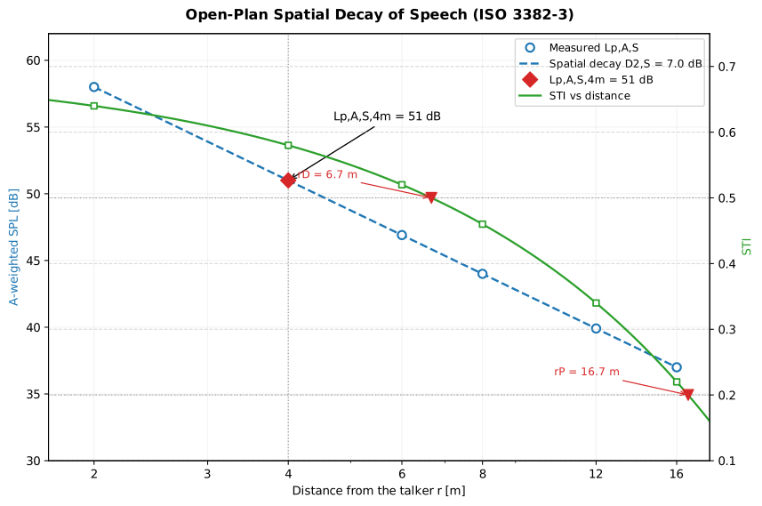
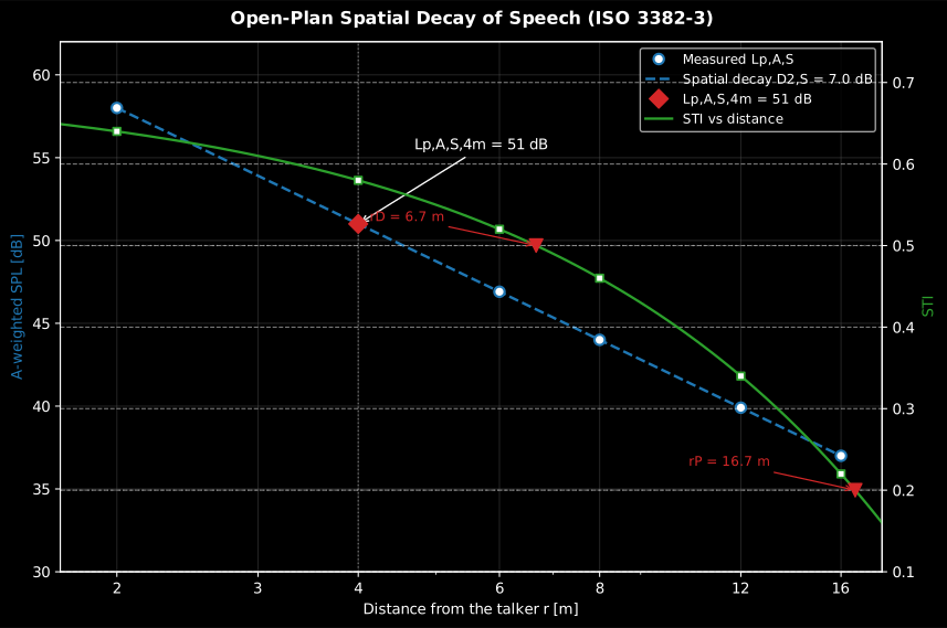
with $L_{p,A,S,4m}$ read off the same line at 4 m. The distraction distance $r_D$ (STI = 0.50) and privacy distance $r_P$ (STI = 0.20) come from a linear regression of STI against distance.

Both distances are read off the fitted line, and clause 6.3 allows the reading to fall outside the measured span — Figure 3 b) draws the line extended to the crossing. So an $r_D$ that lands inside the line is a measurement, while an $r_P$ well beyond the last position is an extrapolation whose confidence decays with distance: quote it with the measured span alongside (”$r_P$ = 17 m, extrapolated from positions to 16 m”). The standard also anticipates offices where the STI never falls to 0.20 — “it can prove impossible to determine the privacy distance if STI > 0,20 in all positions” — and that is what a nan means here, not a bug. A non-decreasing STI along the line usually means the last position sat near a reflecting wall, where both level and STI rise; clause 6.2 says to discard that position from the $D_{2,S}$ and $r_D$ fits rather than to puzzle over it.

ISO 3382-3 Annex A is informative, but it fixes the two ends of the scale:

Quantity	Typical poor office	Good target
$D_{2,S}$	< 5 dB	≥ 7 dB
$L_{p,A,S,4m}$	> 50 dB	≤ 48 dB
$r_D$	> 10 m	≤ 5 m

Those ranges are informative, and national guidance or the client brief overrides them. Read $D_{2,S}$ and $L_{p,A,S,4m}$ as a pair: the decay rate is a slope and the 4 m level is its offset, so quoting either alone flatters or condemns the room.

$L_{p,A,B}$ is the fourth required quantity and it is not decoration: the background noise is measured in octave bands at every position with the same $\ge 10$ s integration, A-weighted, and averaged over the line, and that average is the masker the per-position STI is computed against. Spatially averaging it is what keeps $r_D$ and $r_P$ unambiguous. It is also why open-plan design has two levers rather than one — attenuation (screens, an absorptive ceiling, layout: these raise $D_{2,S}$ and lower $L_{p,A,S,4m}$) and masking (raising the background so speech loses intelligibility sooner) — and why the office is measured furnished, unoccupied and with the services running. An office measured with the ventilation or the masking system turned down returns a higher STI at every position and pushes both distances outward by metres with nothing having changed in the room.

import numpy as np
from phonometry import room

# A stand-in line: the levels are built to a clean 7 dB per doubling and the
# STI to a straight -0.03 per metre, so every printed number can be checked
# by hand. A measured line is not this tidy (see below).
r = np.array([2.0, 4.0, 6.0, 8.0, 12.0, 16.0])       # distances from the talker (m)
lp = 65.0 - 7.0 * np.log2(r)                          # A-weighted speech level (dB)
sti = 0.70 - 0.03 * r                                 # STI per position

m = room.open_plan_metrics(r, lp, sti)
print(round(m.d2s, 1), round(m.lp_as_4m, 1))         # 7.0 dB, 51.0 dB
print(round(m.rd, 1), round(m.rp, 1))                # 6.7 m, 16.7 m
m.plot()   # the spatial-decay regression of the figure below

Reading this office. $D_{2,S}$ = 7.0 dB is exactly the Annex A good-office threshold, but $L_{p,A,S,4m}$ = 51.0 dB is above the 50 dB poor line, and $r_D$ still lands at 6.7 m. It is a good decay rate spent from too high a starting level, so the fix is attenuation near the talker — a screen, an absorptive ceiling raft over the workstation — rather than more decay further out. And a measured line does not look like this one: positions scatter about the fitted line, typically by one to two decibels, with the near ones pulled up by the direct field and the far ones flattened by the background floor. What is reported is the regression, not any single position: $L_{p,A,S,4m}$ is read off the line even when no microphone stood at 4 m, which is also why six positions are preferred — four barely constrain a slope once one of them has to be discarded.

Show the code for this figure

import matplotlib.pyplot as plt
import numpy as np
from phonometry import room

r = np.array([2.0, 4.0, 6.0, 8.0, 12.0, 16.0])       # distances from the talker (m)
lp = 65.0 - 7.0 * np.log2(r)                          # A-weighted speech level (dB)
sti = 0.70 - 0.03 * r                                 # STI per position
m = room.open_plan_metrics(r, lp, sti)

# One line: the D2,S regression rebuilt from the result fields, with the
# rD / rP crossings marked (the figure above adds the measured points and
# the STI axis on top of it):
m.plot()
plt.show()

import matplotlib.pyplot as plt
import numpy as np
from phonometry import room

r = np.array([2.0, 4.0, 6.0, 8.0, 12.0, 16.0])       # distances from the talker (m)
lp = 65.0 - 7.0 * np.log2(r)                          # A-weighted speech level (dB)
sti = 0.70 - 0.03 * r                                 # STI per position
m = room.open_plan_metrics(r, lp, sti)

# Spatial decay: measured Lp,A,S vs distance on a log axis, the D2,S
# regression rebuilt from the result fields, and STI with the rD / rP
# crossings on a twin axis:
b = -m.d2s / np.log10(2.0)                 # regression slope vs lg(r)
a = m.lp_as_4m - b * np.log10(4.0)         # intercept from the 4 m level
rr = np.logspace(np.log10(2.0), np.log10(16.0), 100)

fig, ax = plt.subplots()
ax.semilogx(r, lp, "o", label="Measured Lp,A,S")
ax.semilogx(rr, a + b * np.log10(rr), "--", label=f"D2,S = {m.d2s:.1f} dB")
ax.plot(4.0, m.lp_as_4m, "D", label=f"Lp,A,S,4m = {m.lp_as_4m:.0f} dB")
ax.set_xlabel("Distance from the talker r [m]")
ax.set_ylabel("A-weighted speech level [dB]")
ax.set_xlim(1.8, 20.0)

twin = ax.twinx()
twin.semilogx(r, sti, "s-", color="#2ca02c", label="STI")
twin.axvline(m.rd, ls=":", color="#2ca02c")
twin.axvline(m.rp, ls=":", color="#9467bd")
twin.annotate(f"rD = {m.rd:.1f} m", (m.rd, 0.52))
twin.annotate(f"rP = {m.rp:.1f} m", (m.rp, 0.22))
twin.set_ylabel("STI")
twin.set_ylim(0.0, 1.0)

lines, labels = ax.get_legend_handles_labels()
tl, tlab = twin.get_legend_handles_labels()
ax.legend(lines + tl, labels + tlab, loc="best")
plt.show()

Against the Annex A scale, that one office sits between two very different rooms:

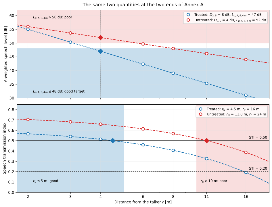
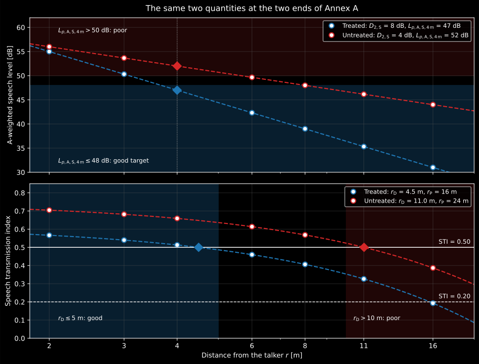
The two ends of Annex A on one axis. The treated office meets all three targets; the untreated one misses all three, and its privacy distance — 24 m read off a 16 m line — is exactly the extrapolation warned about above.

Show the code for this figure

import matplotlib.pyplot as plt
import numpy as np
# `room` is the import of the first snippet above.

positions = np.array([2.0, 3.0, 4.0, 6.0, 8.0, 11.0, 16.0])
for d2s, lp_4m, sti_0, sti_slope in ((8.0, 47.0, 0.62, 0.0267),
                                     (4.0, 52.0, 0.75, 0.0227)):
    slope = -d2s / np.log10(2.0)
    levels = (lp_4m - slope * np.log10(4.0)) + slope * np.log10(positions)
    res = room.open_plan_metrics(positions, levels, sti_0 - sti_slope * positions)
    print(round(res.d2s, 1), round(res.lp_as_4m, 1),
          round(res.rd, 1), round(res.rp, 1))
    # 8.0 47.0 4.5 15.7   /   4.0 52.0 11.0 24.2
    plt.semilogx(positions, levels, "o--")
plt.show()

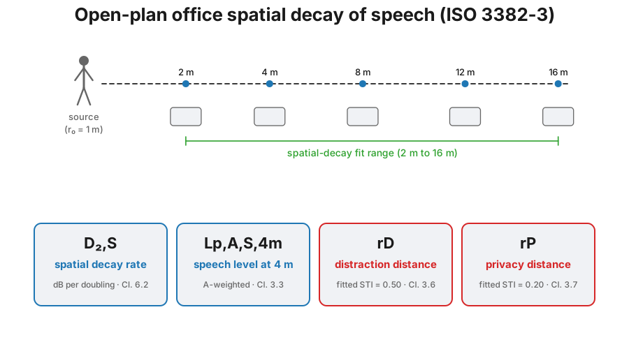
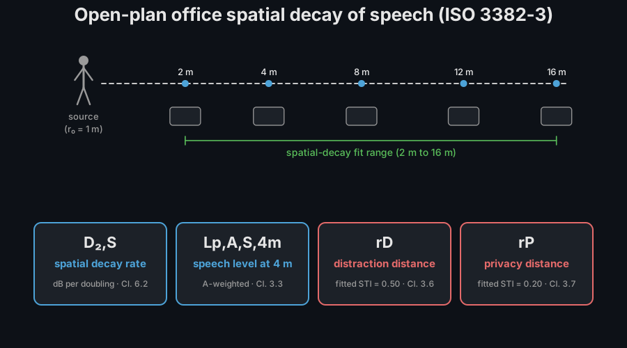
The line itself is worth a to-scale plan. plot_open_plan_geometry draws the source, the microphone line across the workstations and the two distances on the axis, and a result that retained its positions redraws its own line with m.plot_geometry().

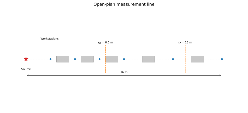
Every ISO 3382-3 quantity comes off this one line: six microphones from 2 m to 16 m through the workstations, with $r_D$ and $r_P$ landing between them.

Show the code for this figure

import matplotlib.pyplot as plt
from phonometry import room

# The 2-16 m line of the example, with the distraction and privacy
# distances marked on the axis.
room.plot_open_plan_geometry([2.0, 4.0, 6.0, 8.0, 12.0, 16.0],
                             rd=6.5, rp=13.0)
plt.show()

# A result retains its positions, so m.plot_geometry() draws its own
# line with the regressed rD and rP.

Measuring the line

Clauses 5.1 and 5.2 fix everything the drawing above leaves implicit.

The source (5.1.1). An omnidirectional loudspeaker radiating pink noise, meeting the omnidirectionality requirements of ISO 3382-1 — the standard is explicit about why: people in an open-plan office do not continuously speak in any fixed direction. A deterministic pink-spectrum signal (an MLS or a sweep, acquired as in the room impulse response guide) is an accepted substitute, and the results are derived from the impulse response. Its sound power is verified as in ISO 3382-1, with the source at 1.2 m, and clause 6.2 sets the level: high enough in each octave band that the pink noise exceeds the background by 6 dB at the most distant position.

The receiving chain (5.1.2). A sound level meter meeting IEC 61672-1 class 1, an omnidirectional microphone (including whatever is attached to it), and octave filters to IEC 61260. If the signal is recorded for off-line processing, the whole chain has to comply.

The room condition (5.2.1). Measured furnished, with nobody present but the operators, and with the HVAC and any sound-masking system running at the power of a typical working day. The standard states the failure directly: if the sources run at reduced power the STI values come out too high, which overestimates both $r_D$ and $r_P$. Because people are absent, the masking that real conversation provides is not in the measurement either, so the actual distances in use are shorter than the measured ones.

The line (5.2.2). It crosses the workstations and need not be straight. 6 to 10 successive positions are preferred and 4 is the minimum, with the first at the nearest workstation. Source and microphone both stand at head height in a workstation, 1.2 m above the floor — standing working positions are out of scope — and at least 0.5 m from tables and 2.0 m from walls and other reflecting surfaces. At least two source positions are used; if only one line is possible, it is measured with two sources firing in opposite directions. Where the ceiling or the furniture changes, the office is treated as separate zones, each with its own set of single numbers.

What is recorded at each point (5.2.3). Four things: the octave-band pink-noise level, the STI, the octave-band background level, and the distance to the source — over 125 Hz to 8 kHz, with an integration time of at least 10 s (longer for non-stationary background such as traffic).

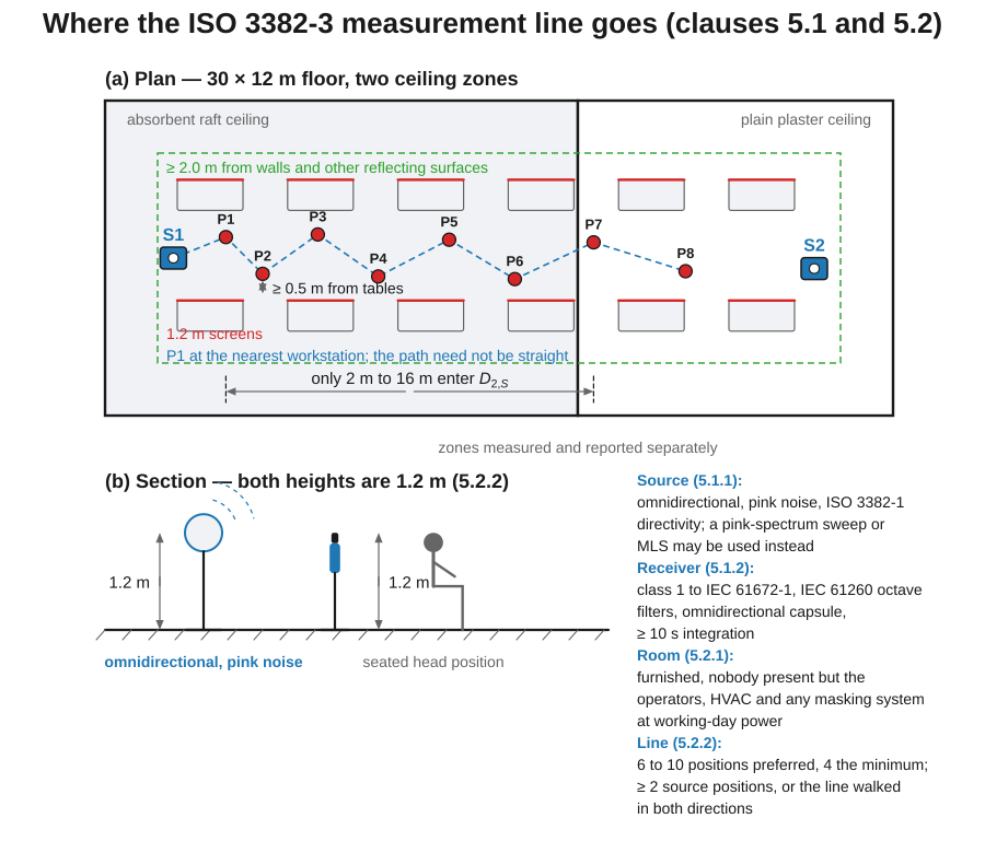
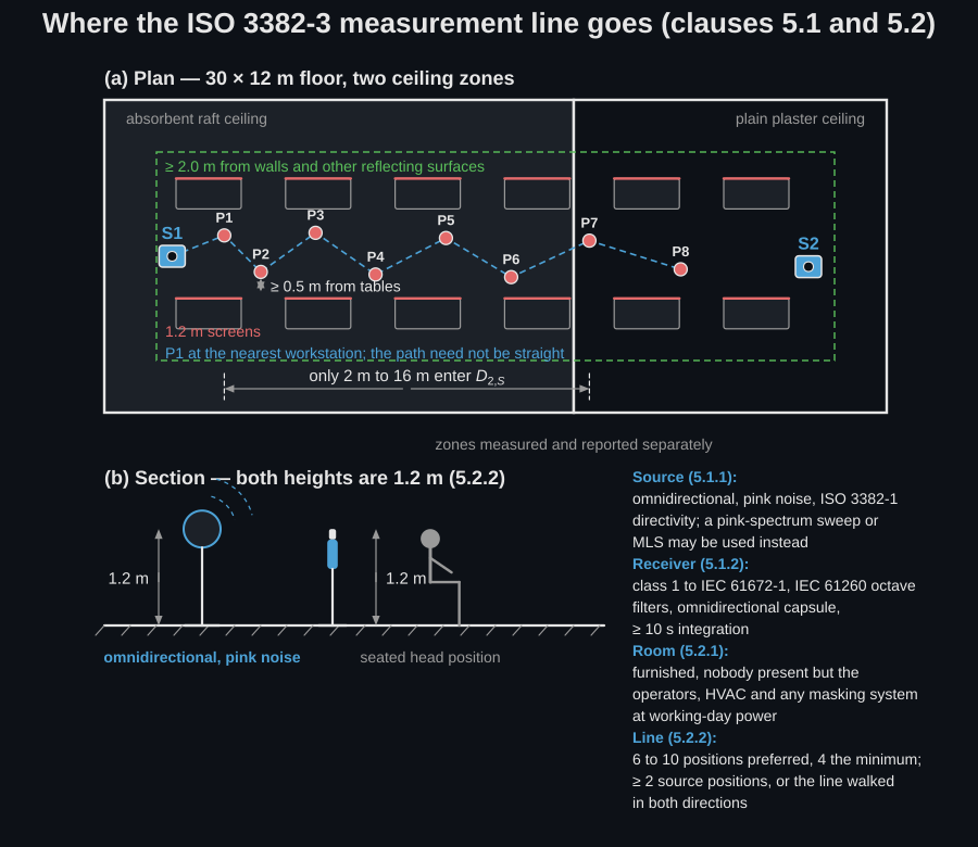
Why the window stops at 2 m and 16 m. Clause 6.2 admits only positions between 2 m and 16 m into the $D_{2,S}$ regression, and both ends have a reason. Nearer than 2 m the receiver sits in the talker’s direct field, whose 6 dB per doubling is a property of free space rather than of the office; beyond 16 m the speech level has normally reached the background, so the regression would be fitting noise. A line of six positions from 2 m to 16 m therefore keeps at least four points inside the fit even if the last one has to be discarded for sitting near a wall.

From the measured pink noise to $L_{p,A,S,n}$

A loudspeaker is not a talker, so ISO 3382-3 never uses its level directly. Clause 6.2 measures the room with pink noise and then re-clothes the result in the spectrum of a real voice. What is kept from each position is not its absolute level but the band-by-band attenuation relative to the source at 1 m (Eq. 1-2), so the loudspeaker’s output level cancels out and only has to sit far enough above the background:

$$L_{p,Ls,1m,i}\approx L_{W,Ls,i}-11\text{dB},D_{n,i}=L_{p,Ls,1m,i}-L_{p,Ls,n,i}.$$

That attenuation is then applied to the normal-effort speech spectrum (Eq. 3), A-weighted and summed energetically over the seven octave bands (Eq. 4):

$$L_{p,S,n,i}=L_{p,S,1m,i}-D_{n,i},L_{p,A,S,n}=10{\log }_{10}\sum _{i}10^{(L_{p,S,n,i}+A_i)/10}.$$

Table 1 supplies the omnidirectional normal-effort spectrum and the A-weightings:

Band $i$	$f$ [Hz]	$L_{p,S,1m,i}$ [dB]	$A_i$ [dB]
1	125	49.9	−16.1
2	250	54.3	−8.6
3	500	58.0	−3.2
4	1000	52.0	0.0
5	2000	44.8	+1.2
6	4000	38.8	+1.0
7	8000	33.5	−1.1

whose A-weighted total is 57.4 dB — a normal talking voice at 1 m.

The A-weighted pink-noise reading on the meter is not the input open_plan_metrics expects. Feeding it in gives an absolute level that is the loudspeaker’s, not a talker’s, so $L_{p,A,S,4m}$ is wrong outright and $D_{2,S}$ is biased by the spectral difference between pink noise and speech. Run the four-step chain first:

import numpy as np
# `room` is the import of the open_plan_metrics block above.

# ISO 3382-3 Table 1: normal-effort unisex speech at 1 m, omnidirectional,
# and the A-weighting, octave bands 125 Hz to 8 kHz.
speech_1m = np.array([49.9, 54.3, 58.0, 52.0, 44.8, 38.8, 33.5])
a_weight = np.array([-16.1, -8.6, -3.2, 0.0, 1.2, 1.0, -1.1])

# Measured octave-band pink-noise levels, one row per measurement position.
pink = np.array([
    [72.0, 71.0, 70.0, 69.0, 67.0, 64.0, 60.0],
    [67.0, 66.0, 64.5, 63.0, 60.5, 57.0, 52.5],
    [63.5, 62.0, 60.0, 58.0, 55.0, 51.0, 46.0],
    [60.0, 58.5, 56.0, 53.5, 50.0, 45.5, 40.0],
])
source_1m = np.full(7, 90.0) - 11.0        # Eq. (1): Lp,Ls,1m = Lw,Ls - 11 dB

d_n = source_1m - pink                     # Eq. (2): attenuation per band
speech_n = speech_1m - d_n                 # Eq. (3): re-clothed in speech
lp_a_s = 10 * np.log10(np.sum(10 ** ((speech_n + a_weight) / 10), axis=1))
print(np.round(lp_a_s, 1))                 # [48.  42.4 37.8 33.8]  Eq. (4)

dist = np.array([2.0, 4.0, 8.0, 16.0])
chain = room.open_plan_metrics(dist, lp_a_s, 0.70 - 0.03 * dist)
print(round(chain.d2s, 1), round(chain.lp_as_4m, 1))     # 4.7 42.9

The band arithmetic itself — A-weighting and energetic summation — is the same as in Levels.

open_plan_metrics() parameters

Parameter	Type	Units	Range / default	Notes
positions_m	1D array	m	≥ 4 positions, all > 0	Source-to-receiver distances
spl_a_speech	1D array	dB	same length	A-weighted speech level $L_{p,A,S,n}$ per position, from the Clause 6.2 Eq. (1)-(4) chain — not the measured pink-noise dB(A)
sti_values	1D array	—	same length	STI per position (full IEC 60268-16 method)

Returns an OpenPlanResult with d2s, lp_as_4m, rd and rp; its .plot() redraws the Clause 6.2 spatial-decay regression from those four fields and marks rd / rp. d2s/lp_as_4m are nan if fewer than two positions fall in 2–16 m; rd/rp are nan when STI does not decrease with distance. The per-position STI can itself be measured with the STIPA tools in the Speech Transmission Index guide.

ISO 3382-3 report (.report())

OpenPlanResult.report(path) renders a one-page PDF fiche laid out like an open-plan-office speech-privacy measurement report: a standard-basis line, an optional metadata header block, a compact metrics table of the four quantities open_plan_metrics returns ($D_{2,S}$, $L_{p,A,S,4m}$, the distraction distance $r_D$ and the privacy distance $r_P$) stacked above the full-width spatial-decay plot (.plot(), the Clause 6.2 regression on the logarithmic distance axis with the 4 m read-off and the $r_D$ / $r_P$ crossings marked, the Figure 3 style curve), the boxed $D_{2,S}$ with the other quantities alongside, and a footer with the fixed disclaimer. ISO 3382-3 characterises a space rather than defining an intrinsic pass/fail, so a verdict row appears only when a target spatial decay rate is supplied through the metadata’s requirement field (ReportMetadata(requirement=...), read as the minimum acceptable $D_{2,S}$ in dB, reflecting the informative quality ranges of Annex A where a larger spatial decay is better; the room passes at or above it). It uses the same ReportMetadata container and rendering engine as the ISO 3382-1/-2 room-acoustics fiche; the open-plan-specific fields area (floor area), source_positions and receiver_positions (the number of measurement positions) populate the header, alongside client, test_room (the office or zone), specimen (the description and furnishing state), instrumentation, temperature, relative_humidity, pressure, measurement_standard, test_date, laboratory, operator, report_id and notes. Passing metadata=None produces a bare characterisation fiche. The fiche embeds the spatial-decay chart, so rendering needs both reportlab and matplotlib (pip install "phonometry[report,plot]"); only engine="reportlab" is supported. The fiche renders in English by default; pass language="es" for a Spanish fiche (translated fixed strings and a comma decimal separator).

import numpy as np
from phonometry import room, ReportMetadata

r = np.array([2.0, 3.0, 4.0, 6.0, 8.0, 11.0, 16.0])   # distances from the talker (m)
# Another stand-in line, built to a clean 7 dB per doubling as above; a
# measured one scatters about the fit by a decibel or two.
lp = 62.0 - 7.0 * np.log2(r)                           # A-weighted speech level (dB)
sti = 0.65 - 0.03 * r                                  # STI per position

result = room.open_plan_metrics(r, lp, sti)
result.report(
    "open_plan_fiche.pdf",
    metadata=ReportMetadata(
        test_room="Open-plan office B",
        specimen="Furnished, unoccupied, background noise present",
        area=420.0, source_positions=2, receiver_positions=7,
        measurement_standard="ISO 3382-3",
        temperature=22.0, relative_humidity=45.0,
        laboratory="Phonometry Reference Laboratory",
        requirement=7.0,          # adds a verdict against a target D2,S
    ),
)                                 # D2,S + Lp,A,S,4m, rD, rP and the decay curve

The example fiche is regenerated with make reports and kept rendered in the repository; click the preview to open the PDF.

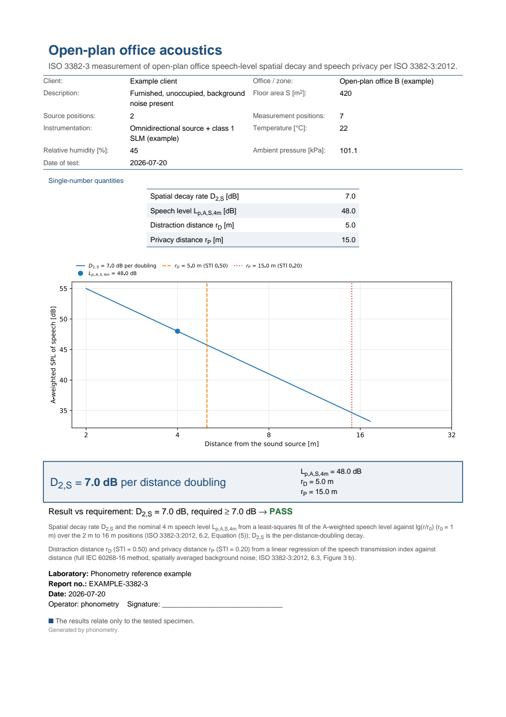
One-page open-plan-office fiche: a metadata header (client, office/zone, description, floor area, source and measurement positions, instrumentation, temperature, humidity and pressure), the metrics table of the four single-number quantities (D2,S = 7.0 dB per doubling, Lp,A,S,4m = 48.0 dB, rD = 5.0 m, rP = 15.0 m) above the spatial-decay plot on a logarithmic distance axis with the D2,S regression, the 4 m read-off and the rD and rP crossings, the boxed D2,S, and a PASS verdict against the 7.0 dB target.

Download the report (PDF)

Open-plan office acoustics fiche (OpenPlanResult.report): D2,S, Lp,A,S,4m, rD, rP and the spatial-decay curve.

Crowd self-noise in an occupied room

ISO 3382-3 above measures an office. The complementary question at design time is a prediction: in a room whose only noise source is its own occupants, how loud does the background get, and does conversation still work? Long (Architectural Acoustics 2e, Ch. 17, Eqs. (17.50) to (17.54)) sets the two competing levels at a listener. The signal is the direct field of the person across the table,

$$L_p(\text{signal})=L_W+10{\log }_{10}\left[\frac{Q}{4\pi r^2}\right],$$

and the noise is the reverberant field that $N$ simultaneous talkers build up,

$$L_p(\text{noise})=L_W+10{\log }_{10}N+10{\log }_{10}\left[\frac{4}{N{A}_{\text{tab}}}\right],$$

with $L_W$ the sound power level of one talker (about 70 dB in normal conversation), $Q$ the talker’s forward directivity (about 2), $r$ the talker-to-listener distance and $A_{\text{tab}}$ the equivalent absorption area per occupied table, so $N{A}_{\text{tab}}$ is the room’s total absorption.

from phonometry import room

# Long's hard restaurant: about 20 metric sabins, a talker at Lw = 70 dB,
# a listener 1.2 m away across the table.
print(round(room.speech_direct_level(1.2)))          # 60 dB direct field
print(round(room.crowd_noise_level(1, 20.0)))        # 63 dB with one talker
print(round(room.crowd_noise_level(20, 20.0)))       # 76 dB with 20 tables

# An alpha 0.9 ceiling over the 13.7 x 13.7 m room adds 170 metric sabins.
print(round(room.crowd_noise_level(20, 20.0 + 170.0)))   # 66 dB

Subtracting the two gives the speech-to-noise ratio, and this is the result worth remembering:

$$L_{SN}=10{\log }_{10}\left[\frac{Q}{4\pi r^2}\right]+10{\log }_{10}\left[\frac{A_{\text{tab}}}{4}\right].$$

Neither $L_W$ nor $N$ survives. A busier room is not intrinsically worse, because each new table brings both a talker and its own share of absorption. What decides whether a restaurant works is the absorption per table, not the absorption of the room. Requiring $L_{SN}>-6$ dB for adequate cross-table communication at a separation $r_s$, and $L_{SN}<-9$ dB so a neighbouring table $r_t$ away is not overheard, turns into a pair of design bounds (Eqs. (17.53) and (17.54)):

$$A_{\text{tab}}>6.31r_s^2,A_{\text{tab}}<3.16r_t^2(Q=2).$$

Caution

The first constant is printed as 6.33. The closed form above, at the same $Q=2$ that yields Long’s own second constant 3.16 exactly, gives 6.31, and his prose (“6.3 or more square metres, 68 sq ft”) converts to 6.317 m². The library computes both bounds from the speech-to-noise ratio rather than hardcoding either constant, so they stay mutually consistent; the misprint is recorded in the errata registry.

from phonometry import room

print(round(room.absorption_per_table(1.0, -6.0), 2))   # 6.31 m2 per table at 1 m
print(round(room.absorption_per_table(2.5, -9.0), 1))   # 19.8 m2 at 2.5 m spacing

# A real layout: 1.2 m across the table, 2.0 m to the next one.
print(round(room.absorption_per_table(1.2, -6.0), 2))   # 9.09 m2, the floor
print(round(room.absorption_per_table(2.0, -9.0), 2))   # 12.66 m2, the ceiling

crowd = room.crowd_noise([20.0, 95.0, 190.0], distance=1.2)
crowd.plot()      # self-noise vs occupancy, against the -6 dB limit

The two bounds are a window, and it can be empty. Requiring $6.31r_s^2<A_{\text{tab}}<3.16r_t^2$ means the window exists only when $r_t/r_s>\sqrt{6.31/3.16}\approx 1.41$: pack the tables closer than that and there is no absorption at all that lets you converse across your own table without being overheard at the next one. The layout above passes, with $r_t/r_s=1.67$ and 3.6 m² of room between the bounds.

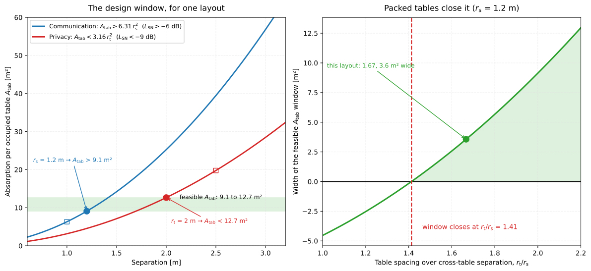
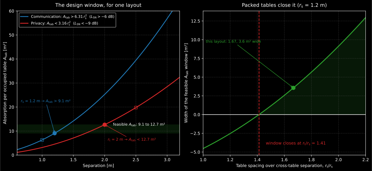
Left: for one layout the two inequalities leave a band of feasible absorption per table. Right: how wide that band is as the tables move apart — below $r_t/r_s=1.41$ it has negative width, which is the geometric statement that conversation and privacy have become incompatible whatever the ceiling is made of.

Show the code for this figure

import matplotlib.pyplot as plt
import numpy as np
# `room` is the import of the block above.

span = np.linspace(0.6, 3.2, 200)
plt.plot(span, room.absorption_per_table(span, -6.0), label="communication")
plt.plot(span, room.absorption_per_table(span, -9.0), label="privacy")

r_s, r_t = 1.2, 2.0
lower = float(room.absorption_per_table(r_s, -6.0))
upper = float(room.absorption_per_table(r_t, -9.0))
plt.axhspan(lower, upper, alpha=0.2)
print(round(upper - lower, 1), round(r_t / r_s, 2))     # 3.6 1.67
print(round(float(np.sqrt(6.31 / 3.16)), 2))            # 1.41: the closure ratio
plt.legend(); plt.show()

Where $A_{\text{tab}}$ itself comes from. For a room that exists, measure the reverberation time to ISO 3382-2 and invert Sabine, $A=0.161V/T$ — the same convention ISO 354 defines — with the room impulse response and Room Acoustics guides supplying $T$. For a room being designed, take it off surface by surface as in Sound absorption in enclosed spaces. Either way $A_{\text{tab}}=A/N$ with $N$ the number of simultaneously occupied tables — not the covers, and not the tables installed. That is what makes a half-full restaurant a different room from a full one at the same absorption, and it is why adding tables at fixed absorption is what pushes a room past its limit. It also means a T30 measured in the empty room is enough to predict how it will sound full.

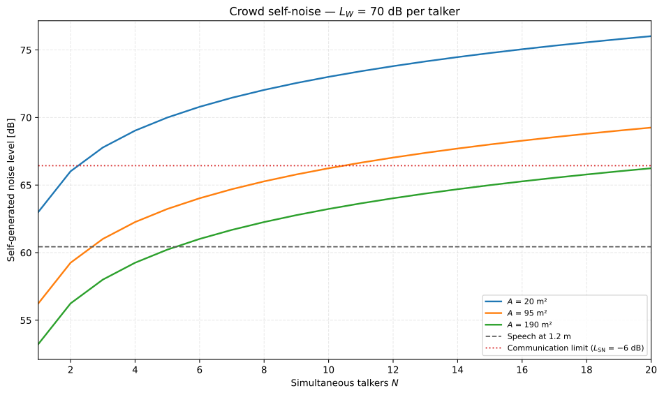
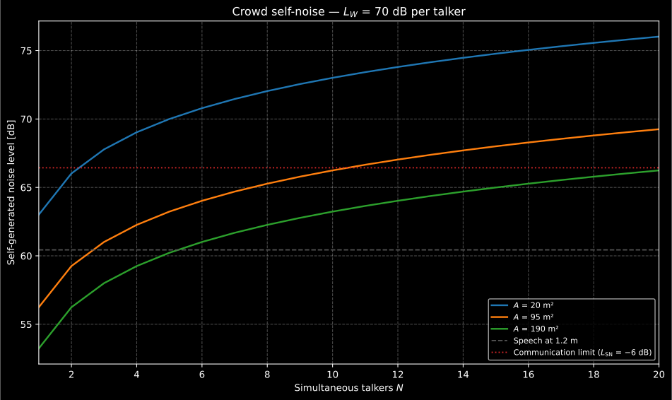
The same 20 talkers in three rooms. The hard room (20 m² of absorption) crosses the communication limit before the fourth table is occupied; adding the absorptive ceiling of Long’s example (190 m² in total) keeps all 20 tables below it. The curves are parallel because occupancy always costs $10{\log }_{10}N$: only the vertical offset, which is the absorption, is a design variable.

Show the code for this figure

import matplotlib.pyplot as plt
import numpy as np
from phonometry import room

# One line — the occupancy sweep straight from the result:
result = room.crowd_noise([20.0, 95.0, 190.0], distance=1.2)
result.plot()
plt.show()

# Or draw it by hand from Equation (17.51):
n = np.arange(1, 21)
fig, ax = plt.subplots()
for area in (20.0, 95.0, 190.0):
    ax.plot(n, room.crowd_noise_level(n, area), label=f"A = {area:.0f} m²")
signal = room.speech_direct_level(1.2)
ax.axhline(signal, ls="--", label="Speech at 1.2 m")
ax.axhline(signal + 6.0, ls=":", label="Communication limit")
ax.set(xlabel="Simultaneous talkers N", ylabel="Self-generated noise level [dB]")
ax.legend()
plt.show()

crowd_noise() parameters

Parameter	Type	Units	Range / default	Notes
absorption_areas	float or 1D array	m²	> 0	Total room absorption areas to compare
talkers	1D array, optional	—	≥ 1, default 1..20	Occupancy axis $N$
distance	float	m	> 0, default 1.2	Talker-to-listener distance $r$
sound_power_level	float	dB re 1 pW	default 70	Talker $L_W$
directivity	float	—	> 0, default 2	Talker $Q$

Returns a CrowdNoiseResult (talkers, absorption_areas, levels, signal_level, communication_level, speech_to_noise()) with .plot(). The pieces speech_direct_level, crowd_noise_level, speech_to_noise_ratio and absorption_per_table are callable directly.

What this guide covers

• Covered

  ISO 3382-3:2012 Clause 4 and Clause 6.2/6.3 open-plan quantities ($D_{2,S}$, $L_{p,A,S,4m}$, $r_D$, $r_P$) from room.open_plan_metrics, with the to-scale measurement-line drawing (room.plot_open_plan_geometry and .plot_geometry()) and the one-page ISO 3382-3 fiche through .report(). The clause 5.1 and 5.2 measurement conditions and the Annex A quality ranges are quoted here for planning and reading. Long’s Architectural Acoustics 2e Chapter 17 crowd self-noise model (Eqs. (17.50) to (17.54)) through room.crowd_noise and its parts, with the Eq. (17.53)-(17.54) design window and its closure condition.

• Not covered

  ISO 3382-3’s per-position STI is taken as an input to open_plan_metrics rather than computed inside it: measure it with the STIPA tools of the Speech Transmission Index guide. The fourth required single number, the average A-weighted background noise $L_{p,A,B}$, is likewise not computed here — it is the energetic A-weighted average of the per-position octave-band background levels, and it belongs in the report alongside the three this page produces. Nothing checks the measurement conditions of clauses 5.1 and 5.2 either: the function consumes distances, levels and STI values wherever they came from, so the source directivity, the furnished-and-unoccupied state and the background capture are the operator’s responsibility, not the library’s. The implemented edition is frozen at ISO 3382-3:2012; the superseding ISO 3382-3:2022 revision removes the privacy distance $r_P$, adds the comfort distance $r_C$ and moves the per-position STI to the indirect IEC 60268-16 method, and is not the one checked here. The crowd self-noise model is a design calculation and deliberately does not model the Lombard reflex: it cancels out of $L_{SN}$ as long as everyone raises their voice equally, so the model explains why the level spirals upward in a hard room rather than predicting where it stops. It also assumes a diffuse reverberant field and a single absorption figure per table, so it says nothing about screens, local absorption or where in the room a given table sits.

See also

• Room Acoustics: the ISO 3382-1/2 decay parameters of the same room.
• Measuring the Room Impulse Response: the acquisition behind the per-position levels.
• Speech Transmission Index: the STI/STIPA measurement that feeds the per-position sti_values.
• Speech Intelligibility Index: the ANSI S3.5 view of the same intelligibility question.
• Levels: the A-weighted levels behind the spatial decay.
• Theory: the room-acoustic derivations this page builds on.
• API reference: room.open_plan.
• Theory: Impulse response and room-acoustic parameters: the decay and absorption theory the ISO 3382-3 distraction distance is measured against.

References

• International Organization for Standardization. (2012). Acoustics — Measurement of room acoustic parameters — Part 3: Open plan offices (ISO 3382-3:2012). The open-plan speech-privacy quantities this page implements. Since revised as ISO 3382-3:2022 (https://www.iso.org/standard/77437.html); the 2012 edition is the implemented one.
• Long, M. (2014). Architectural acoustics (2nd ed.). Academic Press. https://doi.org/10.1016/C2012-0-03257-5The crowd self-noise model of Chapter 17, Equations (17.50) to (17.54).