Reverberation-time prediction (Sabine, Eyring, Arau)

The reverberation time $T$, the time for the sound-energy level to fall by 60 dB after the source stops, is predicted here from a room’s volume, boundary areas and the sound-absorption coefficients of its surfaces, through the classical statistical-acoustics formulae. This is the design-stage counterpart of the measured reverberation time of Room acoustics (ISO 3382) and complements the EN 12354-6 model of Sound absorption in enclosed spaces, which specialises the same physics to that standard’s Clause 4.

phonometry offers five models, ordered by how much they account for a non-uniform absorption distribution:

Model	How the absorption enters	Best for
Sabine	absorption term $A={\sum }_i{S}_i{\alpha }_i$	low, uniform absorption
Eyring (Norris-Eyring)	absorption term $-S\ln (1-\bar{\alpha })$	strong, uniform absorption
Millington-Sette	absorption term $-{\sum }_i{S}_i\ln (1-{\alpha }_i)$	a few very absorptive surfaces
Fitzroy	area-weighted arithmetic mean of three axial Eyring times	anisotropic rooms
Arau-Puchades	area-weighted geometric mean of the same three	anisotropic rooms (author-preferred)

The first three models differ only in the denominator of $T=kV/(\text{term}+4mV)$, with the Sabine constant $k=24\ln 10/c_0$ (so $k=0.161$ for $c_0=343m/s$) and the air-absorption term $4mV$. Fitzroy and Arau-Puchades work differently: they compute three axial Eyring times and combine those, so their entries are reverberation times and cannot be substituted into that denominator (§2).

EN 12354-6 pins the same constant differently. It rounds $24\ln 10$ to 55.3 and fixes $c_0=345.6m/s$ so that the factor is exactly the traditional 0.16, which makes the enclosed-space model return reverberation times about 0.7 % shorter than sabine_reverberation_time for the same room — 0.608 s against 0.612 s for the 8 × 5 × 3 m shoebox of §1. It is a rounding convention, not a physical disagreement: passing speed_of_sound=345.6 to the classical function brings the two within 0.07 %, the residue of rounding $24\ln 10=55.262$ to 55.3.

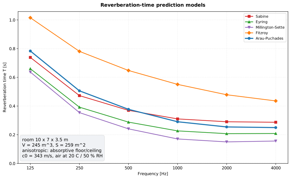
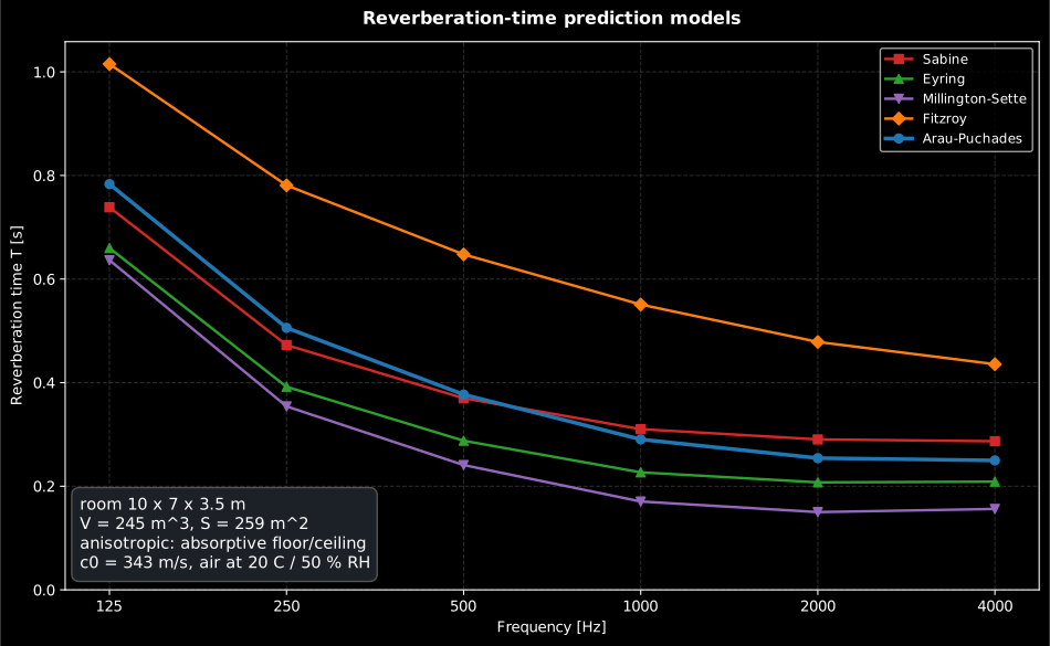
A 10 × 7 × 3.5 m room with a carpeted floor and an acoustic ceiling between hard end walls, run through all five models. Fitzroy sits well above the rest because a single wall pair carries almost all the absorption; Sabine and Eyring bracket the middle, and Arau-Puchades tempers Fitzroy’s over-prediction with a geometric mean. Where the five spread like this, the room is telling you its field is not diffuse (§4) — the spread is the diagnostic, not a defect of one formula.

Show the code for this figure

import matplotlib.pyplot as plt
from phonometry import environment, room

# A 10 x 7 x 3.5 m room: hard end walls, lightly treated side walls and a
# very absorptive floor/ceiling pair (carpet plus an acoustic ceiling).
bands = [125.0, 250.0, 500.0, 1000.0, 2000.0, 4000.0]
alpha_x = [0.06, 0.07, 0.08, 0.09, 0.10, 0.10]
alpha_y = [0.12, 0.14, 0.16, 0.18, 0.20, 0.20]
alpha_z = [0.30, 0.50, 0.65, 0.78, 0.82, 0.80]
m = environment.air_attenuation_m(bands, 20.0, 50.0)   # air at 20 C / 50 % RH
res = room.reverberation_time_models((10.0, 7.0, 3.5),
                                     (alpha_x, alpha_y, alpha_z),
                                     air_attenuation=m, frequencies=bands)
res.plot()   # the five model curves per band
plt.show()

0. Assembling the inputs

All five models consume two things a drawing does not hand you directly: a list of areas with a coefficient each, and — for Fitzroy and Arau-Puchades — one mean coefficient per pair of opposing walls. Almost every wrong prediction is a wrong take-off rather than a wrong formula, so this step deserves as much care as the choice of model.

Areas. Use the internal boundary areas of the room, measured to the finished surfaces, and give every material its own row: a wall carrying a window and a door becomes three rows whose areas sum to the wall. EN 12354-6 Annex E case 3 does exactly this, splitting a 10.90 m² long wall into 9.81 m² lined at ${\alpha }_s$ = 0.85 plus 1.09 m² bare at 0.04. Do not average a lining into its wall by hand; the formulae already do the area weighting, and Millington-Sette does it non-linearly, so pre-averaging changes the answer.

Coefficients. These are random-incidence values measured to ISO 354 on a 10-12 m² sample in a stated mounting, not material constants (Sound Absorption Measurement and Rating). Mounting depth and edge condition change them substantially, so a coefficient quoted for a product bonded direct to the substrate does not describe the same product on a 200 mm plenum. ISO 354 delivers one-third-octave data and an octave-band run takes the arithmetic mean of the three thirds. A datasheet’s single-number rating — ${\alpha }_w$, NRC, SAA — is not a substitute for the per-band table (see the EN 12354-6 guide, which states the prohibition normatively). Audience and seating are rated per square metre of the floor area they occupy, not per person. Feeding reverberation-room data back into Sabine is self-consistent because the ISO 354 coefficient is defined through Sabine’s formula, which is also why a coefficient above 1.0 is a documented outcome rather than an error (§4).

Wall-pair means. fitzroy_reverberation_time and arau_puchades_reverberation_time take one mean coefficient per opposing pair, in the order $({\bar{\alpha }}_x,{\bar{\alpha }}_y,{\bar{\alpha }}_z)$ where ${\bar{\alpha }}_i$ belongs to the pair perpendicular to axis $i$. Each is the area-weighted mean over both surfaces of the pair. In a shoebox the two surfaces have equal areas, so it reduces to their arithmetic mean — but not once one of them is split by a window or a lining. Absorption that is patchy within one pair (an absorptive wall facing a hard one) is outside both models even though the code still returns a number; that case belongs to §4’s list of failures.

# `room` is the import of the figure block above.
# A 9 x 7 x 3 m classroom (V = 189 m3), 1 kHz octave band, taken off by material.
surfaces = [
    (63.0, 0.05),   # floor, vinyl on concrete
    (63.0, 0.70),   # ceiling, 20 mm acoustic tile
    (12.0, 0.04),   # long wall A: glazing
    (15.0, 0.05),   # long wall A: plaster around the glazing
    (2.0, 0.10),    # long wall B: wooden door
    (25.0, 0.05),   # long wall B: plaster
    (21.0, 0.05),   # short wall, plaster
    (21.0, 0.05),   # short wall, plaster
]
print(round(room.sabine_reverberation_time(189.0, surfaces), 2))   # 0.59 s

def pair_mean(rows):                       # area-weighted mean over one pair
    area = sum(s for s, _ in rows)
    return sum(s * a for s, a in rows) / area

means = (pair_mean(surfaces[6:8]),         # x-pair: the two short walls
         pair_mean(surfaces[2:6]),         # y-pair: the two long walls
         pair_mean(surfaces[0:2]))         # z-pair: floor and ceiling
print([round(a, 3) for a in means])                                # [0.05, 0.05, 0.375]
print(round(room.fitzroy_reverberation_time((9.0, 7.0, 3.0), means), 2))       # 1.33 s
print(round(room.arau_puchades_reverberation_time((9.0, 7.0, 3.0), means), 2)) # 0.76 s

One take-off, both input forms. The spread it produces — 0.59 s from Sabine against 1.33 s from Fitzroy — is not a bug: all of this room’s absorption sits on one wall pair, which is exactly the case §2 exists for and §4 warns about.

1. Sabine, Eyring and Millington-Sette

Every model in the family follows from one picture. In a diffuse field a ray travels a mean free path $4V/S$ between reflections, so it meets a boundary $cS/4V$ times per second and gives up part of its energy each time. Take that loss as $\alpha$ per reflection and linearise it and you get Sabine: the decay rate is proportional to ${\sum }_i{S}_i{\alpha }_i$, and 60 dB of decay takes $kV/A$ seconds. Keep the loss multiplicative instead — after $n$ reflections the energy is down by $(1-\bar{\alpha }{)}^n$ — and the logarithm of that factor gives Eyring’s $-S\ln (1-\bar{\alpha })$, which is why Eyring is always the shorter of the two and why the two converge as $\bar{\alpha }\to 0$. Do the same bookkeeping surface by surface rather than on the mean and you get Millington-Sette, which collapses to zero the moment one surface absorbs perfectly, because a ray that strikes it never returns. The air term $4mV$ is the same path length applied to the medium instead of to the boundary.

The three statistical models take the room volume and a list of (area, absorption_coefficient) surfaces. Sabine is exact only for low, uniform absorption; Eyring replaces the absorption area by $-S\ln (1-\bar{\alpha })$ and is correct where Sabine overestimates $T$; Millington-Sette sums the Eyring term surface by surface, so a single perfectly absorbing surface drives $T$ to zero.

$$T_{\text{Sab}}=\frac{kV}{{\sum }_i{S}_i{\alpha }_i},T_{\text{Eyr}}=\frac{kV}{-S\ln (1-\bar{\alpha })},T_{\text{Mil}}=\frac{kV}{-{\sum }_i{S}_i\ln (1-{\alpha }_i)}.$$

from phonometry import room

# A shoebox 8 x 5 x 3 m (V = 120 m3, S = 158 m2), uniform alpha = 0.2.
surfaces = [(40.0, 0.2), (40.0, 0.2), (24.0, 0.2),
            (24.0, 0.2), (15.0, 0.2), (15.0, 0.2)]
print(round(room.sabine_reverberation_time(120.0, surfaces), 3))            # 0.612 s
print(round(room.eyring_reverberation_time(120.0, surfaces), 3))            # 0.548 s
print(round(room.millington_sette_reverberation_time(120.0, surfaces), 3))  # 0.548 s

For a uniform distribution Eyring and Millington-Sette coincide, and both fall below Sabine; Sabine’s over-estimate at high absorption is the reason Eyring exists. As $\alpha \to 0$, Eyring reduces to Sabine. Air absorption enters every model through the power (intensity) attenuation coefficient $m$, in neper per metre:

from phonometry import environment, room

m = environment.air_attenuation_m(2000.0, temperature=20.0, relative_humidity=50.0)
surfaces = [(40.0, 0.3), (40.0, 0.3), (24.0, 0.3),
            (24.0, 0.3), (15.0, 0.3), (15.0, 0.3)]
print(round(room.eyring_reverberation_time(120.0, surfaces, air_attenuation=m), 3))
# 0.337 s, against 0.343 s with the air term omitted

Six milliseconds on a third of a second is why the air term is usually ignored in a room this size, and it is a scaling argument rather than a rule of thumb: $4mV$ grows with the volume while the boundary term grows with the area, so the air’s share rises with the room’s linear dimension. In the same 120 m³ room the 2 kHz correction is 1.9 %; in a 20 000 m³ concert hall with $\bar{\alpha }=0.15$ the 4 kHz Eyring time falls from 4.31 s to 2.49 s at 20 °C / 50 % RH — 42 % — and to 1.52 s if the hall is dry at 20 % RH. That is the second half of the behaviour: $m$ rises steeply with frequency and falls with humidity, so the driest condition is the worst case and a hall that measures well in a humid summer can sound noticeably brighter in winter. The coefficient itself comes from the ISO 9613-1 atmospheric absorption model, evaluated at the room’s own temperature and humidity.

Every statistical model also assumes a diffuse field, and low frequencies break that assumption first: below the Schroeder frequency $f_s\approx 2000\sqrt{T/V}$ ($V$ in m³, $T$ in s — 141 Hz for a 200 m³ classroom with $T$ = 1 s) the room responds as a set of discrete modes, not as a reverberant mixture. room.schroeder_frequency(T, V) computes it, and the modes of a rectangular room enumerate what is down there. The 2D FDTD simulation below drives a rigid 5 m by 3.5 m room exactly on its (2,1) mode and then between two modes; the standing-wave pattern that builds up on resonance is what Sabine and Eyring cannot see.

A 2D FDTD simulation of a rigid 5 by 3.5 metre room driven at the 84 Hz (2,1) mode and at an off-mode frequency side by side. On resonance a standing-wave pattern with fixed nodal lines grows until it dominates the RMS pressure map; off resonance the forced response stays weak and never organises into that nodal structure.

Download the animation (WebM)

A 2D FDTD simulation of a rigid 5 by 3.5 metre room driven at the 84 Hz (2,1) mode and at an off-mode frequency side by side. On resonance a standing-wave pattern with fixed nodal lines grows until it dominates the RMS pressure map; off resonance the forced response stays weak and never organises into that nodal structure.

Download the animation (WebM)

2. Fitzroy and Arau-Puchades (anisotropic rooms)

When the absorption is concentrated on one axis (a carpeted floor and an acoustic ceiling against otherwise hard walls), a single mean $\bar{\alpha }$ misrepresents the field. Fitzroy and Arau-Puchades split a rectangular (shoebox) room into the three pairs of opposing walls and combine the axial Eyring reverberation times $T_i$ (each using the whole surface $S$ and the mean absorption ${\bar{\alpha }}_i$ of the wall pair perpendicular to axis $i$):

$$T_{\text{Fitz}}=\sum _i\frac{S_i}{S}{T}_i(\text{arithmetic}),T_{\text{Arau}}=\prod _i{T}_i^{S_i/S}(\text{geometric}).$$

Each $T_i$ has a physical reading: it is the reverberation time the room would have if every one of its boundaries absorbed like the wall pair on axis $i$, so it is the decay experienced by sound bouncing predominantly along that axis — which is why the formula uses the whole surface $S$ and not $S_i$. The weight $S_i/S$ is then the fraction of the boundary that steers energy into that axis. A shoebox with a soft floor and ceiling between hard walls therefore has three coexisting decay rates, and the two models differ only in how they blend them: Fitzroy averages them arithmetically, so the slowest axis dominates and the result runs high when one pair is very reflective; Arau-Puchades averages them geometrically, which lets the fastest axis pull the answer down. Both assume a rectangular room and absorption uniform within each pair, so a room with one absorptive wall facing a hard one of the same pair is outside the model even though the code still returns a number (§0).

from phonometry import room

# 8 x 5 x 3 m room, absorptive x-wall pair (alpha 0.5), hard elsewhere (0.1).
dims = (8.0, 5.0, 3.0)
absorption = (0.5, 0.1, 0.1)   # mean alpha of the (x, y, z) wall pairs
print(round(room.arau_puchades_reverberation_time(dims, absorption), 3))  # 0.812 s
print(round(room.fitzroy_reverberation_time(dims, absorption), 3))        # 0.974 s

By the arithmetic-geometric-mean inequality the Arau-Puchades time never exceeds the Fitzroy time; Fitzroy is known to over-predict when one wall pair is very reflective, which is why Arau-Puchades recommends the geometric mean. Both reduce exactly to Eyring for a uniform absorption distribution.

The misrepresentation these two models exist for can be run as an experiment, and the clip below does. One flat 8 × 2.5 m section is simulated twice with the same total statistical absorption: spread over all four edges, or concentrated on the floor-and-ceiling pair (the carpeted floor and acoustic ceiling of this page’s own example, α ≈ 0.79) between hard ends. Any formula built on a single mean $\bar{\alpha }$ sees the same number in both rooms, so the Sabine and Eyring predictions — evaluated for the two-dimensional section, whose mean free path is $\pi S/P$ — form one band shared by both. The spread room decays inside it, a straight line at T = 160 ms against Sabine’s 201. The concentrated room’s decay has no single slope, 183 ms early and 236 ms late, and it finishes 10 dB above its twin; the surviving field is visible in the RMS panel as a standing pattern between the hard ends, nearly uniform from floor to ceiling — sound running parallel to the absorber, brushing it at grazing incidence instead of striking it, which is the field §4 describes in disproportionate rooms.

A 2D FDTD simulation of a flat 8 by 2.5 metre section run twice with the same total statistical absorption, spread over all four edges or concentrated on the floor and ceiling between hard ends. A lower axis races the two measured energy decays through the shared Sabine-Eyring band: the spread room decays inside the band at 160 ms, the concentrated room shows two slopes of 183 and 236 ms and finishes 10 dB louder, and its RMS map keeps a striped grazing field running parallel to the absorbing pair.

Download the animation (WebM)

A 2D FDTD simulation of a flat 8 by 2.5 metre section run twice with the same total statistical absorption, spread over all four edges or concentrated on the floor and ceiling between hard ends. A lower axis races the two measured energy decays through the shared Sabine-Eyring band: the spread room decays inside the band at 160 ms, the concentrated room shows two slopes of 183 and 236 ms and finishes 10 dB louder, and its RMS map keeps a striped grazing field running parallel to the absorbing pair.

Download the animation (WebM)

3. Comparing the five models per band

reverberation_time_models builds the six boundary surfaces of a rectangular room from its dimensions and the three wall-pair mean absorptions, then evaluates all five models on a common footing and returns a ReverberationModelResult whose .plot() draws the figure above.

from phonometry import room

# 10 x 7 x 3.5 m room, absorptive floor/ceiling against harder walls.
res = room.reverberation_time_models(
    (10.0, 7.0, 3.5),
    (
        [0.06, 0.07, 0.08, 0.09, 0.10, 0.10],   # x-pair: hard end walls
        [0.12, 0.14, 0.16, 0.18, 0.20, 0.20],   # y-pair: lightly treated walls
        [0.30, 0.50, 0.65, 0.78, 0.82, 0.80],   # z-pair: carpet + acoustic ceiling
    ),
    frequencies=[125.0, 250.0, 500.0, 1000.0, 2000.0, 4000.0],
)
print(res.sabine.round(2))         # [0.74 0.47 0.37 0.31 0.3  0.3 ]
print(res.arau_puchades.round(2))  # [0.79 0.51 0.38 0.29 0.26 0.27]
print(res.fitzroy.round(2))        # [1.02 0.79 0.66 0.57 0.51 0.51]
res.plot()   # the five model curves per band (the figure above)

Show the code for this figure

import matplotlib.pyplot as plt
from phonometry import environment, room

m = environment.air_attenuation_m([125.0, 250.0, 500.0, 1000.0, 2000.0, 4000.0], 20.0, 50.0)
room.reverberation_time_models(
    (10.0, 7.0, 3.5),
    (
        [0.06, 0.07, 0.08, 0.09, 0.10, 0.10],
        [0.12, 0.14, 0.16, 0.18, 0.20, 0.20],
        [0.30, 0.50, 0.65, 0.78, 0.82, 0.80],
    ),
    air_attenuation=m,
    frequencies=[125.0, 250.0, 500.0, 1000.0, 2000.0, 4000.0],
).plot()
plt.show()

Sabine and Eyring are the two workhorses, and the per-band spread between them is itself a diagnostic. The diagram runs the room of this section through both, with the validity boundary every statistical formula shares.

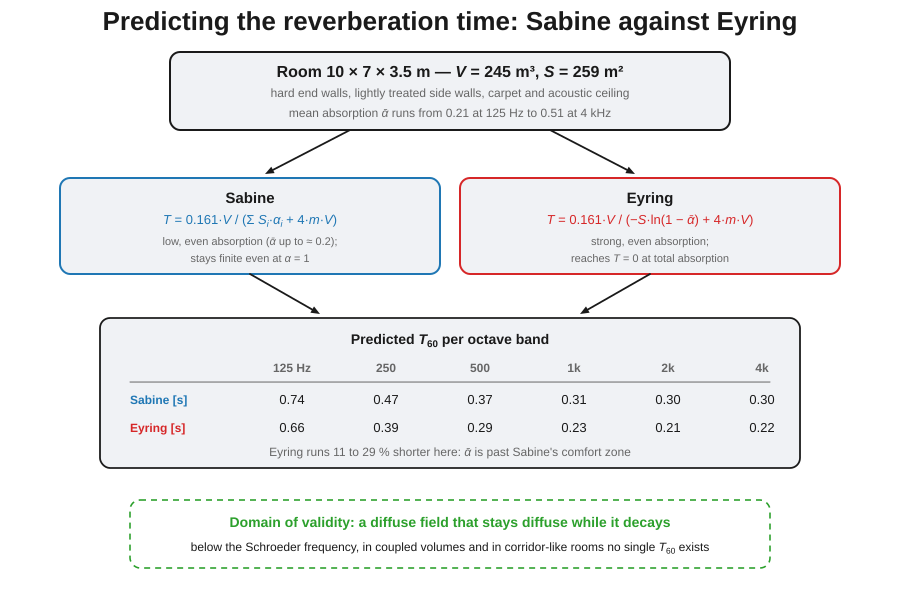
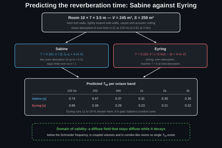
The same 245 m³ room through Sabine and Eyring alone. Eyring reads 11 % shorter at 125 Hz and 29 % shorter at 4 kHz, because its correction grows with the mean absorption, which here rises from 0.21 to 0.51 across the spectrum. The closing note is the domain both share.

4. Choosing a model, and when every model fails

The single axis along which the first three models disagree is the mean absorption, so it is worth seeing them plotted against it before reading the bullets below.

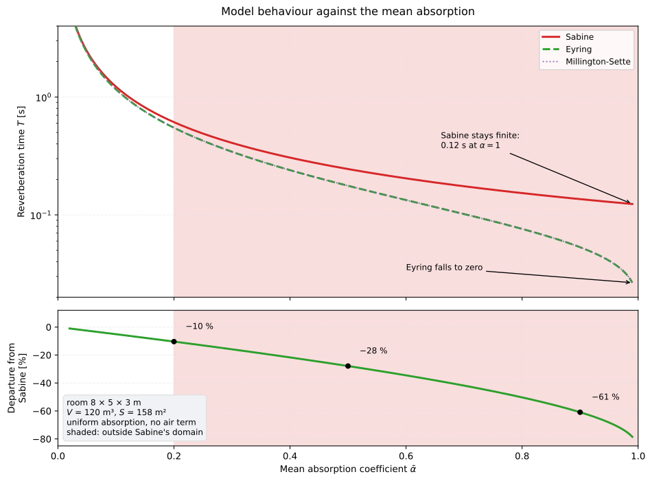
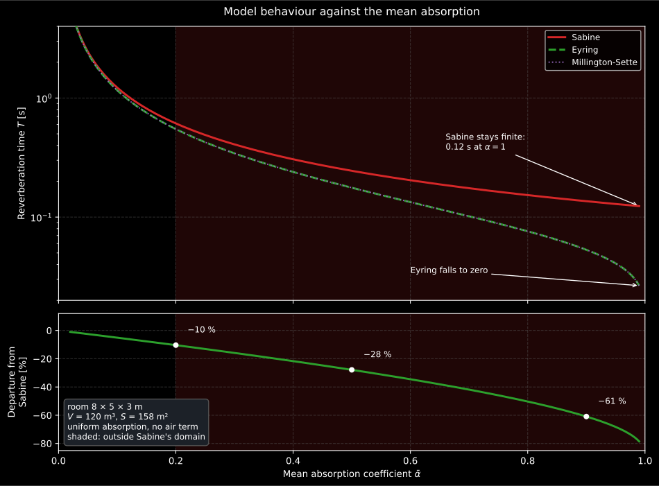
A 8 × 5 × 3 m shoebox with a uniform mean absorption swept from 0.02 to 0.99. Below $\bar{\alpha }\approx 0.1$ all three coincide, which is why Sabine survived a century of use. Eyring and Millington-Sette are identical for a uniform distribution and fall away from Sabine as the absorption rises: −10 % at $\bar{\alpha }$ = 0.2, −28 % at 0.5, −61 % at 0.9. At the right-hand edge the structural difference is visible — Sabine still predicts a finite 0.12 s for a room with an opening in every direction, while the logarithmic models reach zero.

Show the code for this figure

# `room` and `plt` are the imports of the figure block at the top of the page.
import numpy as np

alpha = np.linspace(0.02, 0.99, 200)
volume, area = 120.0, 158.0
sab = np.array([room.sabine_reverberation_time(volume, [(area, a)]) for a in alpha])
eyr = np.array([room.eyring_reverberation_time(volume, [(area, a)]) for a in alpha])

fig, (top, bottom) = plt.subplots(2, 1, sharex=True)
top.semilogy(alpha, sab, label="Sabine")
top.semilogy(alpha, eyr, "--", label="Eyring")
top.set_ylabel("T [s]")
top.legend()
bottom.plot(alpha, 100.0 * (eyr / sab - 1.0))
bottom.set_xlabel(r"Mean absorption $\bar\alpha$")
bottom.set_ylabel("Departure from Sabine [%]")
plt.show()

The five formulae are not rivals on a single axis of accuracy; each has a domain of validity:

• Sabine is the tool for live rooms with low, reasonably even absorption (mean $\bar{\alpha }$ up to roughly 0.2): classrooms, halls, reverberation chambers. It is also the convention wired into measurement practice, because the ISO 354 absorption coefficient is defined through Sabine’s formula, so feeding reverberation-room data back into Sabine is self-consistent even where the formula is strained. Its structural defect shows at high absorption: with $\alpha =1$ on every surface (an opening in every direction) it still predicts a finite reverberation time.
• Eyring is the choice for evenly treated rooms with substantial absorption: studios, treated offices, listening rooms. It reaches $T=0$ for total absorption, and its correction over Sabine grows with $\bar{\alpha }$ (about 10 % shorter at $\bar{\alpha }=0.2$, 30 % at 0.5).
• Millington-Sette handles a mix of very absorptive and hard surfaces better than a single mean, but it is meant for measured, sub-unity coefficients: a single surface with ${\alpha }_i=1$ drives the whole prediction to zero. Reverberation-room coefficients at or above 1.0 are a documented ISO 354 outcome — edge diffraction scatters more energy into the sample than its flat area intercepts, see Sound Absorption Measurement and Rating — and they lie outside the domain of the logarithmic term. To use Millington-Sette anyway you must bring the coefficient into $[0,1)$, and that is a modelling decision the formula does not prescribe: whatever adjustment you choose (limiting to just below 1 is common), record it alongside the prediction.
• Fitzroy and Arau-Puchades target shoebox rooms whose absorption is concentrated on one axis, the typical office or dwelling with a soft floor and ceiling between hard walls. Arau’s geometric mean tempers Fitzroy’s known over-prediction when one wall pair is very reflective.

What each model accepts. phonometry enforces each formula’s own domain, so an out-of-domain coefficient raises a ValueError rather than returning a meaningless number:

Model	Accepts	Why
Sabine	any ${\alpha }_i\ge 0$, including above 1	the linear sum ${\sum }_i{S}_i{\alpha }_i$ stays finite
Eyring	individual ${\alpha }_i$ above 1, provided $\bar{\alpha }<1$	only the mean enters $\ln (1-\bar{\alpha })$
Millington-Sette	every ${\alpha }_i<1$	its per-surface $\ln (1-{\alpha }_i)$ diverges at 1
Fitzroy	each wall-pair mean $<1$	the means are the inputs, and each enters a logarithm
Arau-Puchades	each wall-pair mean $<1$	same

All five reject a coefficient above 2.0 outright, on the grounds that it is a percentage passed as a fraction: measured ISO 354 values do not exceed about 1.2.

When every formula fails. All five inherit the same assumption: a diffuse field, with sound arriving equally from all directions at every point, that stays diffuse while it decays. The common breakages:

• Below the Schroeder frequency the band holds a handful of discrete modes (the animation in §1) and a statistical reverberation time is not defined at all; each mode decays at its own rate set by the wall impedances it actually touches.
• Coupled volumes (a hall with an open stage house, two rooms through a doorway) produce double-slope decays; no single $T$ exists, and the measured T20 and T30 disagree (the curvature diagnostic of the room-parameter guide).
• Disproportionate rooms (corridors, low flat halls) with the absorption on one surface pair keep a grazing sound field parallel to the hard surfaces that the absorber barely touches; the measured time can be up to twice any statistical prediction, the practical experience recorded in EN 12354-6 (see Sound absorption in enclosed spaces). That grazing field is the striped survivor of the §2 clip, which measures it outliving the whole Sabine-Eyring band of its own section.
• Focusing geometries (domes, curved rear walls) concentrate late energy instead of mixing it, producing position-dependent decays no single-number formula can represent.

Scattering objects restore the mixing the models assume: a furnished room follows the statistical prediction distinctly better than the same room bare, beyond what the furniture’s own absorption area accounts for. The clip below is that mechanism with the absorption taken out of it, so only the mixing is left: an 800 Hz wavefront enters a 4 m rigid-walled hall filled with rigid columns 10 to 17 cm across, a quarter to two fifths of the 42.9 cm wavelength. Every column diffracts the front and sheds a scattered wavelet, the wavelets interfere, and within a few passes the specular front has become energy spread over the whole hall with no preferred direction — which is the assumption Sabine and Eyring both start from, arriving here as a result rather than as a hypothesis. Nothing in the hall absorbs, so what you are watching is only the redistribution; the decay at the end is the energy draining out through the two open ends.

An 800 Hz plane wavefront sweeps a 4 m rigid-walled hall filled with a staggered colonnade of rigid columns 10 to 17 cm across, simulated at 2.5 mm; every column diffracts the front and sheds a scattered wavelet, and the wavelets interfere until the whole hall is filled with structured energy that then drains through the absorbing ends.

Download the animation (WebM)

An 800 Hz plane wavefront sweeps a 4 m rigid-walled hall filled with a staggered colonnade of rigid columns 10 to 17 cm across, simulated at 2.5 mm; every column diffracts the front and sheds a scattered wavelet, and the wavelets interfere until the whole hall is filled with structured energy that then drains through the absorbing ends.

Download the animation (WebM)

In practice, quote a band of predictions (Sabine and Eyring, or Fitzroy and Arau-Puchades for axial cases) rather than a single value; where the models spread, the room is telling you its field is not diffuse.

What value to aim at

A prediction is only useful against a target, and a reverberation-time requirement is a range across the octave bands, not a single upper limit — which is why the fiche of §5 prints the target as a reference line and emits no verdict. Anchors worth carrying:

• Speech-critical rooms (classrooms, meeting rooms, lecture theatres) land between roughly 0.4 s and 0.8 s at mid frequencies, tightening as the room gets smaller. ANSI/ASA S12.60-1:2010 Table 1 is the strictest widely used version of that: for unoccupied, furnished core learning spaces it caps the average of the 500 Hz, 1 kHz and 2 kHz octaves at 0.6 s up to 283 m³ and 0.7 s from 283 m³ to 566 m³, with no requirement above that, and it additionally asks the smaller rooms to be adaptable down to 0.3 s.
• Open-plan offices, corridors and stairwells are specified by absorption area rather than by reverberation time, because the field in them is too far from diffuse for a single $T$ to describe (this is EN 12354-6 clause 4.5’s own advice, and the ISO 3382-3 quantities of Open-Plan Office Acoustics replace $T$ entirely).
• Music rehearsal and performance spaces need more than 1 s and rise with volume; ISO 3382-1 Table A.1 quotes 1.0 s to 3.0 s as the typical EDT range of unoccupied concert and multi-purpose halls up to 25 000 m³.

Two shape rules go with the numbers. The target is normally read at the 500 Hz and 1 kHz octaves, and the goal across frequency is a flat spectrum: a low-frequency rise of more than about 20 % over the mid-frequency value is what makes a treated room sound boomy even when it passes at 500 Hz, and a rise of that size is tolerated in music spaces but not in classrooms. And because the prediction band is often 20 to 30 % wide — the §0 classroom spans 0.59 s to 1.33 s — a design that only just meets its target on the most favourable model has no margin at all.

5. Prediction report (.report())

ReverberationModelResult.report(path) renders a one-page PDF fiche of the prediction: a basis line marking it a design-stage prediction by the five statistical-acoustics models, an optional metadata header block (client, room, description, room volume, total surface area, climate), a per-band table with one reverberation-time column per model beside the model comparison plot (.plot()), and the boxed mid-frequency reverberation time from Arau-Puchades (the recommended model for a non-uniform absorption distribution) with the per-model spread alongside. It is a prediction, not a measurement: the five models bracket the reverberation time likely to occur, so no PASS/FAIL verdict is emitted. A target reverberation time supplied through the metadata’s requirement field is printed as a reference line only, since a room reverberation time is a target range rather than a strictly higher/lower-is-better quantity. It uses the same ReportMetadata container and rendering engine as the other fiches; passing metadata=None produces a bare prediction fiche. Rendering needs reportlab and, for the figure the fiche embeds, matplotlib (pip install "phonometry[report,plot]"); only engine="reportlab" is supported. The fiche renders in English by default; pass language="es" for a Spanish fiche (translated fixed strings and a comma decimal separator).

from phonometry import reverberation_time_models, ReportMetadata

result = reverberation_time_models(
    (8.0, 5.0, 3.0),                       # a shoebox room, one treated wall pair
    ([0.10, 0.15, 0.30, 0.45, 0.55, 0.60], # treated wall pair, per octave band
     [0.08, 0.10, 0.12, 0.15, 0.18, 0.20], # side walls
     [0.05, 0.08, 0.10, 0.12, 0.15, 0.18]),# floor/ceiling
    frequencies=[125.0, 250.0, 500.0, 1000.0, 2000.0, 4000.0],
)
result.report(
    "reverberation_fiche.pdf",
    metadata=ReportMetadata(
        specimen="Classroom, one wall lined with a broadband absorber",
        test_room="Classroom C1",
        temperature=20.0, relative_humidity=50.0,
        laboratory="Phonometry Reference Laboratory",
        requirement=0.8,          # printed as a target reference line, no verdict
    ),
)                                 # the five-model table + the boxed T_mid

The example fiche is regenerated with make reports and kept rendered in the repository; click the preview to open the PDF.

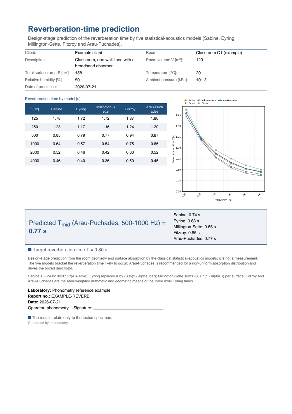
One-page reverberation-time prediction fiche: a metadata header (client, room, description, room volume, total surface area, temperature, humidity and pressure), the octave-band table with one reverberation-time column per model (Sabine, Eyring, Millington-Sette, Fitzroy and Arau-Puchades from 125 Hz to 4 kHz) beside the five-model comparison plot, the boxed mid-frequency reverberation time from Arau-Puchades with the per-model spread alongside, and a target reverberation-time reference line (no PASS/FAIL verdict).

Download the report (PDF)

Reverberation-time prediction fiche (ReverberationModelResult.report), the five-model table and the boxed T_mid.

What this guide covers

• Covered

  The classical statistical-acoustics reverberation-time formulae of Sabine (1922), Eyring (1930), Millington-Sette (1932), Fitzroy (1959) and Arau-Puchades (1988), each with its own domain-of-validity check and the ISO 9613-1-derived air-absorption term, via room.sabine_reverberation_time, room.eyring_reverberation_time, room.millington_sette_reverberation_time, room.fitzroy_reverberation_time, room.arau_puchades_reverberation_time and the combined room.reverberation_time_models.

• Not covered

  EN 12354-6’s own Clause 4 model (a Sabine calculation with an added object term and the ISO 9613-1 air term) is a distinct, standard-defined calculation that lives in the Sound absorption in enclosed spaces guide, not here. None of the five formulae here models coupled volumes, disproportionate rooms or focusing geometries: their double-slope or position-dependent decays fall outside every diffuse-field assumption (§4). For a measured decay that shows those symptoms, use the T20/T30 curvature diagnostic of the Room Acoustics guide rather than a statistical prediction.

See also

• Sound Absorption Measurement and Rating: the ISO 354 measurement every ${\alpha }_s$ on this page comes from, its mounting dependence, and the ISO 11654 rating that must not be substituted for the per-band table (§0).
• Room acoustic parameters (ISO 3382-1/2): the measured counterpart, and the curvature diagnostic that tells you a prediction’s diffuse-field assumption has failed.
• Modes of a rectangular room: what is below the Schroeder frequency, where none of these five formulae applies.
• API reference: room.reverberation_prediction and environment.propagation.air_absorption.
• Theory: Sound insulation and absorption, predicted: the diffuse-field assumption every Sabine-family formula makes, and where it stops holding.

References

• Arau-Puchades, H. (1988). An improved reverberation formula. Acustica, 65(4), 163-180. The geometric-mean combination of §2 (its Formula 18). The linked record is the publisher page at Ingenta.
• Carrión Isbert, A. (1998). Diseño acústico de espacios arquitectónicos. Edicions UPC. A Spanish-language textbook treatment of the reverberation models and their use in room design. ISBN 978-84-8301-252-9.
• European Committee for Standardization. (2003). Building acoustics — Estimation of acoustic performance of buildings from the performance of elements — Part 6: Sound absorption in enclosed spaces (EN 12354-6:2003). The classical formulae predate the normative world and enter it through this standard, whose Clause 4 model is a Sabine calculation with object and air terms; see the enclosed-space absorption guide. The linked catalogue record is the BSI Knowledge page for BS EN 12354-6:2003.
• Everest, F. A. (2001). Master handbook of acoustics (4th ed.). McGraw-Hill. The Fig. 7-22 worked example the conformance suite reproduces: Example 1, an untreated 23.3 × 16 × 10 ft room, whose six printed Sabine reverberation times the SI implementation reproduces to ≤ 0.02 s, reinforced by hand-computed closed-form values and the model identities (every model collapses to Eyring for uniform absorption; Eyring collapses to Sabine as the absorption tends to zero), which transitively carry that real-data anchor to the whole family. ISBN 978-0-07-136097-5.
• Eyring, C. F. (1930). Reverberation time in "dead" rooms. The Journal of the Acoustical Society of America, 1(2A), 217-241. https://doi.org/10.1121/1.1915175The mean-free-path derivation behind the −S ln(1−ᾱ) term of §1.
• Fitzroy, D. (1959). Reverberation formula which seems to be more accurate with nonuniform distribution of absorption. The Journal of the Acoustical Society of America, 31(7), 893-897. https://doi.org/10.1121/1.1907814The axial split into three wall-pair decays of §2.
• International Organization for Standardization. (1993). Acoustics — Attenuation of sound during propagation outdoors — Part 1: Calculation of the absorption of sound by the atmosphere (ISO 9613-1:1993). The atmospheric-absorption coefficient behind the air term 4mV; see the outdoor propagation guide.
• International Organization for Standardization. (2003). Acoustics — Measurement of sound absorption in a reverberation room (ISO 354:2003). Defines the measured absorption coefficient via Sabine's formula, the self-consistency argument of §4.
• Kuttruff, H. (2016). Room acoustics (6th ed.). CRC Press. https://doi.org/10.1201/9781315372150The diffuse-field theory, its limits and the modern assessment of the classical formulae behind §4.
• Millington, G. (1932). A modified formula for reverberation. The Journal of the Acoustical Society of America, 4(1), 69-82. https://doi.org/10.1121/1.1915588The per-surface logarithmic absorption term of §1.
• Sabine, W. C. (1922). Collected papers on acoustics. Harvard University Press. The original reverberation experiments and the T = 0.161 V/A law of §1. The linked copy is the free scan at the Internet Archive.