Sound Absorption Measurement and Rating
Standards: ISO 354ISO 11654ISO 12999Key references: Cox & D'Antonio 2017
Of all the numbers a materials laboratory produces, the sound-absorption coefficient is the one that travels furthest: it leaves the reverberation room on a datasheet, enters a Sabine estimate, an EN 12354-6 absorption budget or a public-tender requirement, and is rarely questioned again. This guide covers that number’s whole laboratory life. The measurement is ISO 354: a sample of 10 m² to 12 m² on the floor of a reverberation room, two decay times, and Sabine’s formula run backwards to get the random-incidence coefficient per one-third-octave band. The rating is ISO 11654: the spectrum collapsed into the weighted coefficient with its letter class A to E, the single number absorber datasheets quote. And because a coefficient without an uncertainty is only half a result, ISO 12999-2 supplies the measurement uncertainty of both. The normal-incidence counterpart measured on small samples lives in the impedance tube guide; the closing section here, after the uncertainty, explains when each of the two is the right tool and why the two numbers do not match.
1. Reverberation-room measurement (ISO 354)
Section titled “1. Reverberation-room measurement (ISO 354)”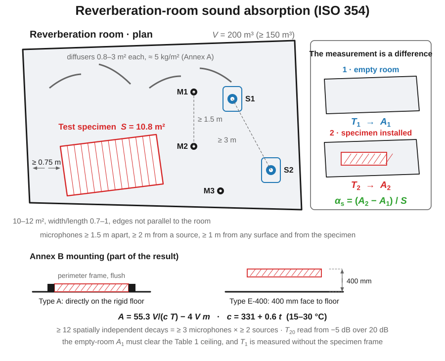
The reverberation-room measurement itself is measure_sound_absorption. It
takes the one-third-octave reverberation time of the empty room () and of
the room with the specimen installed (), the room volume and the
specimen area , and returns a frozen SoundAbsorptionMeasurement. The
equivalent sound absorption areas follow from Sabine’s equation (ISO 354:2003
Eqs. (5) and (7)), and the coefficient from their difference (Eqs. (8)/(9)):
with the speed of sound built from the room air temperature in °C (Eq. (6), valid 15–30 °C) and the power attenuation coefficient of air in 1/m. The coefficient may exceed 1.0 from edge and diffraction effects (Clause 3.7 NOTE 2) and is never clamped; the closing section explains why.
The air-attenuation term , and why the default 0 is not a shortcut.
is a difference of two absorption areas, so a single enters
and identically and the term cancels exactly:
measure_sound_absorption broadcasts one into both, and the default
therefore changes nothing as long as both decays were measured under
the same climate. Only the difference survives, which is why
Clause 6.3.2 asks for and to be measured at almost the same
temperature and relative humidity, inside
and °C throughout the test. The term itself is anything but small:
for the 200 m³ room of the example below at 21.4 °C and 54 % RH, the
ISO 9613-1 attenuation makes about 0.9 m² at 1 kHz, 4.9 m² at 4 kHz and
7.2 m² at 5 kHz; against an empty-room absorption area of about 7.7 m² in
that top band. A few percent of humidity drift between the two runs therefore
moves by more than most of the effect being measured. When the
climate did drift, drop to absorption_coefficient and supply a separate
value per measurement as m1/m2 (with temperature1_c/temperature2_c);
measure_sound_absorption assumes one climate. The per-band comes from
an ISO 9613-1 attenuation in dB/m:
environment.air_attenuation(freqs, temperature_c=21.4, relative_humidity_percent=54.0, atmospheric_pressure_kpa=101.325), converted
with materials.attenuation_from_alpha(alpha),
which is ISO 354’s own .
ISO 354 is a characterisation: it produces the spectrum, not a
single-number rating. The weighted coefficient is an ISO 11654
quantity; feed the measured to weighted_absorption_from_third_octave
in section 3 to obtain it.
import numpy as npfrom phonometry import materials
freqs = np.array([100, 125, 160, 200, 250, 315, 400, 500, 630, 800,                  1000, 1250, 1600, 2000, 2500, 3150, 4000, 5000], float)t_empty = np.array([9.0, 9.0, 8.8, 8.6, 8.4, 8.2, 8.0, 7.8, 7.5, 7.2,                    6.9, 6.6, 6.2, 5.8, 5.4, 5.0, 4.6, 4.2])t_specimen = np.array([8.4, 8.2, 7.7, 7.2, 6.5, 5.7, 4.9, 4.2, 3.6, 3.15,                       2.85, 2.65, 2.55, 2.5, 2.55, 2.6, 2.7, 2.85])
meas = materials.measure_sound_absorption(    freqs, t_empty, t_specimen, volume=200.0, area=10.8, temperature_c=20.0)print(meas.alpha_s[7])   # alpha_s at 500 Hz: 0.328...meas.plot()              # alpha_s versus one-third-octave frequency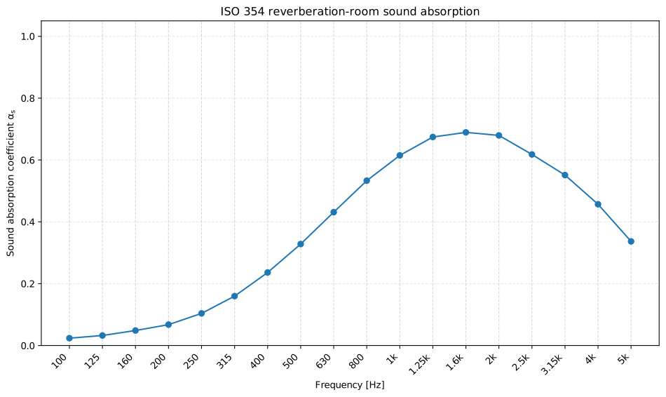
The Sabine inversion of the two decay times: the porous sample barely changes the long low-frequency decays (), bites hardest where its thickness approaches a quarter wavelength, and eases off at high frequency, a typical thin-porous-absorber signature (Cox & D’Antonio 3e, Ch. 5).
Show the code for this figure
import matplotlib.pyplot as pltimport numpy as npfrom phonometry import materials
freqs = np.array([100, 125, 160, 200, 250, 315, 400, 500, 630, 800,                  1000, 1250, 1600, 2000, 2500, 3150, 4000, 5000], float)t_empty = np.array([9.0, 9.0, 8.8, 8.6, 8.4, 8.2, 8.0, 7.8, 7.5, 7.2,                    6.9, 6.6, 6.2, 5.8, 5.4, 5.0, 4.6, 4.2])t_specimen = np.array([8.4, 8.2, 7.7, 7.2, 6.5, 5.7, 4.9, 4.2, 3.6, 3.15,                       2.85, 2.65, 2.55, 2.5, 2.55, 2.6, 2.7, 2.85])meas = materials.measure_sound_absorption(    freqs, t_empty, t_specimen, volume=200.0, area=10.8, temperature_c=20.0)
# One line: the alpha_s spectrum over the one-third-octave band axis.meas.plot()plt.show()
# By hand, from the result's fields:fig, ax = plt.subplots()ax.plot(np.arange(freqs.size), meas.alpha_s, "o-")ax.set_xticks(np.arange(freqs.size))ax.set_xticklabels([f"{f:g}" if f < 1000 else f"{f/1000:g}k" for f in freqs],                   rotation=45)ax.set_xlabel("Frequency [Hz]")ax.set_ylabel("Sound absorption coefficient alpha_s")plt.show()
1.1 How and are actually measured (Clause 7)
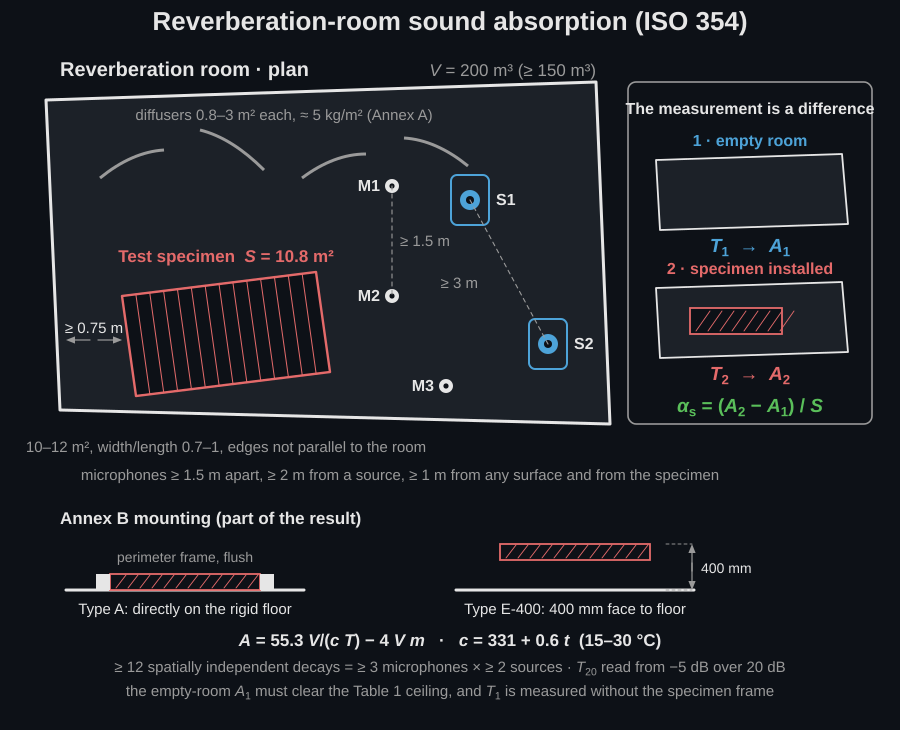
Section titled “1.1 How T1 and T2 are actually measured (Clause 7)”The two reverberation times are ordinary decay measurements (the machinery is the one described under room acoustics), but ISO 354 constrains the geometry and the averaging much harder than a general room survey does, because the whole result is the difference of two numbers that are almost equal at low frequency.
Where the transducers go (Clause 7.1). Both the microphones and the sound source are omnidirectional. Microphone positions are at least 1.5 m apart, 2 m from any sound source and 1 m from any room surface and from the test specimen; source positions are at least 3 m apart. Decay curves measured at different microphone positions shall not be combined in any way: they are separate decays, averaged only as reverberation times.
How many decays (Clause 7.1.4). At least twelve spatially independent decay curves: the number of microphone positions times the number of source positions must reach 12, with a minimum of three microphone positions and two source positions. Several sources may be driven simultaneously if their radiated powers agree within 3 dB in every one-third-octave band, and that buys a reduction to six curves.
How the room is excited (Clause 7.2 or 7.3). Two methods are allowed. The interrupted-noise method drives a loudspeaker with broadband or band-limited noise of continuous spectrum: with broadband noise and a real-time analyser the resulting sound pressure levels must differ by less than 6 dB between adjacent one-third-octave bands, and band-limited noise must be at least one one-third octave wide. The excitation must run long enough to reach the steady state (at least half the expected reverberation time) and start high enough that the bottom of the evaluation range still clears the background by 10 dB. Because a single interrupted decay is a statistical sample, averaging at one microphone/source position is mandatory: at least three decays, and at least ten if the repeatability is to match the other method. The integrated impulse response method (a sweep or a maximum-length sequence deconvolved into the impulse response) is deterministic and needs no averaging at all, which is why it is the method to prefer when the instrumentation allows it.
How each decay is read (Clause 7.4.1). Per band: start 5 dB below the initial level, evaluate over a 20 dB range, and keep the bottom of that range at least 10 dB above the overall background noise: a , extrapolated to 60 dB. and are then the arithmetic mean over all the measurements in that band, carried to at least two decimal places (Clause 8.1.1).
Then do it again. The whole grid is repeated with the specimen installed and nothing else changed: same positions, same excitation, same climate. Any difference between the two runs other than the specimen ends up inside and is reported as absorption.
1.2 The specimen and its mounting (Clause 6.2 and Annex B)
Section titled “1.2 The specimen and its mounting (Clause 6.2 and Annex B)”Geometry (Clause 6.2.1). The test area is between 10 m² and 12 m²; above a room volume of 200 m³ the upper limit is multiplied by , and a weakly absorbing specimen should use the upper limit. The specimen is rectangular with a width-to-length ratio between 0.7 and 1, placed so that no part is closer than 1 m to a room boundary and never closer than 0.75 m, with its edges preferably not parallel to the nearest room edge (both rules exist to keep the specimen out of the pressure maxima at the room boundaries). A heavy specimen may instead stand vertically against a wall resting on the floor, and then the 0.75 m clearance does not apply.
The mounting is part of the result. Annex B is normative and defines the mounting catalogue a datasheet quotes:
| Type | What it is |
|---|---|
| A | Specimen laid or fixed directly against a room surface, normally the reverberation-room floor, with no air space |
| B | Glued to a gypsum board with adhesive dabs and 3 mm shims at the four corners, so a thin air space is retained |
| E-xxx | Mounted over a sealed air space in a fixture of at least 20 kg/m²; the suffix is the distance in millimetres from the exposed face of the specimen to the room surface behind it, tested at E-200, E-300 or E-400 |
| G-xxx | Hung parallel to a room surface (curtains, drapes, blinds); the suffix is again the face-to-surface distance, tested at G-100, other spacings in multiples of 50 mm |
| I | Sprayed or trowelled materials, applied to a substrate and then tested as a Type A with a frame |
| J | Unit absorbers (pads and baffles) in two or three parallel rows over 10 m² to 15 m² of floor, surrounded by a non-absorptive barrier |
The suffix is a cavity depth, and cavity depth moves the answer more than most
material choices do. Predicting the same 50 mm blanket
( kPa·s/m²) with the
multilayer models gives
, class C, laid flat as a Type A, and
, class A, on a Type E-400 mounting. Two classes come from one
product because the 350 mm of air behind it moves the layer into the
particle-velocity maximum at 250 Hz (where the predicted coefficient goes from
0.37 to 0.86). A quoted or without its mounting is
therefore not a material property but an installation result, which is why the
mounting field of the fiche below is not decoration.
The perimeter edge (Annex B.2). The specimen edges shall be sealed or covered so that they do not absorb (unless the product is normally installed with exposed edges, in which case they stay open and the area of the edges is added into ). Either way the treatment goes in the report. Where a reflective frame is used it must be solid rather than hollow, with no air space between frame, specimen and room surface, at least 1.0 mm steel or 12.5 mm gypsum board or wood, tightly butted and sealed, its exposed face flush with the face of the specimen. One consequence is easy to miss: Clause 6.2.1.3 requires the empty-room measurement to be made without the frame or the specimen’s side walls (the barrier of a Type J mounting being the exception), or the frame’s own absorption never cancels out of .
1.3 Is the room fit to measure in? (Clause 6.1 and Annex A)
Section titled “1.3 Is the room fit to measure in? (Clause 6.1 and Annex A)”Three checks decide whether a room may be used at all, and none of them is
performed by this library: measure_sound_absorption only raises an advisory
AbsorptionWarning on the volume and the specimen area.
- Volume and shape (Clauses 6.1.1, 6.1.2). m³, and at least 200 m³ is strongly recommended for a new room; above roughly 500 m³ the high-frequency bands become inaccurate because air absorption dominates the decay. The shape must satisfy , with the longest straight line inside the room (the major diagonal of a rectangular room), and no two room dimensions may stand in the ratio of small whole numbers (both conditions spread the low-frequency modes).
- Empty-room absorption (Clause 6.1.4). shall not exceed the Table 1 ceiling, which is 6.5 m² from 100 Hz to 800 Hz for a 200 m³ room and rises through 7.0 m² at 1 kHz to 14.0 m² at 5 kHz; for another volume the whole table is scaled by . The curve must also be smooth, with no dip or peak differing by more than 15 % from the mean of the two adjacent one-third-octave bands. This is the single check that says the room itself is quiet enough acoustically to see a specimen at all: a leaky, lined or cluttered room spends its absorption budget on itself.
- Diffusivity (Annex A). Diffusers are sheets of low absorption, about 5 kg/m², individually 0.8 m² to 3 m² on one side, slightly curved, randomly oriented and spread through the room; rotating vanes are the alternative, and their rotation frequency must not stand in a small-whole-number ratio to the decay repetition frequency. The qualification procedure of A.2 is empirical: mount a homogeneous porous specimen 5 cm to 10 cm thick whose absorption exceeds 0.9 over 500 Hz to 4000 Hz, measure it with no diffusers, then with about 5 m² of diffusers, then in further 5 m² steps, and plot the mean coefficient over 500 Hz to 5000 Hz against diffuser area. The curve rises and then flattens; the optimum is where it stops rising. In a rectangular room that typically lands at 15 % to 25 % of the room’s total surface area (counting both sides of each diffuser).
What the report must carry (Clause 9). The fiche below holds the specimen
description, , the mounting, , , the temperature and humidity and the
/ and / tables (with verbose=True), that is items (c),
(e) in part, (f) and (g). Four Clause 9 items have no ReportMetadata field
and must be appended by the laboratory: the shape of the room and its total
surface area , the number and size of the diffusers, the number of
microphone and source positions, and the treatment given to the specimen
edges. Results are reported with rounded to 0.1 m² and to
0.01 (Clause 8.3).
ISO 354 report (.report())
Section titled “ISO 354 report (.report())”SoundAbsorptionMeasurement.report(path) renders a one-page PDF fiche laid out
like an accredited reverberation-room absorption test report (ISO 354:2003): a
standard-basis line, a metadata header block, the one-third-octave
table beside the curve (the result’s own .plot()), a boxed
characterisation headline and a footer with the fixed disclaimer. ISO 354 has
no pass/fail verdict and no single-number rating, so the fiche carries neither.
Setting verbose=True adds the reverberation times / and the
equivalent absorption areas / to the table.
It uses the same ReportMetadata container and rendering engine as the other
fiches. The specimen area , room volume , speed of sound , temperature
and humidity are taken from the measurement result (they drove the Sabine
inversion); the descriptive ReportMetadata fields that apply here are
client, manufacturer, specimen, mounting, test_room, test_date,
static_pressure_kpa, measurement_standard, laboratory, operator,
report_id and notes. The requirement field is ignored (ISO 354 has no
verdict). Rendering needs reportlab and, for the figure the fiche embeds,
matplotlib (pip install "phonometry[report,plot]"); only engine="reportlab"
is supported. The fiche renders in English by default; pass language="es" for
a Spanish fiche (translated fixed strings and a comma decimal separator).
from phonometry import materials, ReportMetadata
meas = materials.measure_sound_absorption(    freqs, t_empty, t_specimen, volume=200.0, area=10.8,    temperature_c=20.0, relative_humidity_percent=54.0,)meas.report(    "alpha_s_fiche.pdf",    metadata=ReportMetadata(        specimen="50 mm porous absorber over a 100 mm air gap",        mounting="Type A (against a rigid wall)",        measurement_standard="ISO 354",        test_room="Reverberation room R1",        laboratory="Phonometry Reference Laboratory",    ),)                                  # one-third-octave alpha_s, 100 Hz to 5000 Hz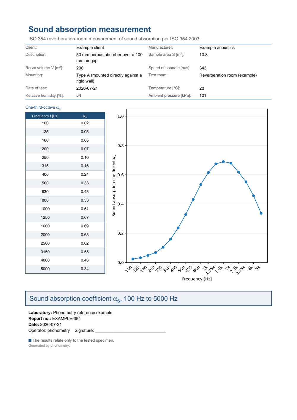
One-page reverberation-room sound absorption fiche: a metadata header (client, specimen, sample area S, room volume V, speed of sound c, mounting, reverberation-room temperature, humidity and pressure), the one-third-octave alpha_s table grouped by octave beside the alpha_s curve, and the boxed characterisation headline over the tested one-third-octave range.
2. The same inversion on bare arrays: absorption_area and absorption_coefficient
Section titled “2. The same inversion on bare arrays: absorption_area and absorption_coefficient”Section 1 returns a whole SoundAbsorptionMeasurement: it carries the room and
specimen metadata, plots itself and renders the ISO 354 fiche. When all that is
wanted is the arithmetic (inside a loop, a fit, a spreadsheet import, or when
the quantity of interest is the room’s own equivalent absorption area rather
than a specimen coefficient), the same Eqs. (5) to (9) are exposed as two plain
array functions. The equivalent absorption area is also what drives ,
, the ISO 3744 environmental correction and the ISO 3741 absorption
term, and absorption_area is the entry point those calculations use.
import numpy as npfrom phonometry import materials
# Third-octave reverberation times of a 200 m^3 room, empty (T1) and with a# 10.8 m^2 absorber sample installed (T2).t1 = np.array([5.0, 4.0, 3.0])t2 = np.array([3.0, 2.5, 2.0])
a_empty = materials.absorption_area(t1, volume=200.0, temperature_c=20.0)print(np.round(a_empty, 2))                    # [ 6.45  8.06 10.75] m^2
alpha = materials.absorption_coefficient(t1, t2, volume=200.0, sample_area=10.8, temperature1_c=20.0)print(np.round(alpha, 3)) # [0.398 0.448 0.498] and are exactly the reverberation times room_parameters returns, so
an ISO 3382-2 decay measurement of the empty and treated room flows straight
into absorption_coefficient.
The result object of section 1 keeps every intermediate of that inversion:
t_empty, t_specimen, absorption_area_empty and
absorption_area_with_specimen. They are worth looking at, because they
show where the method is strong and where it is running out of signal:
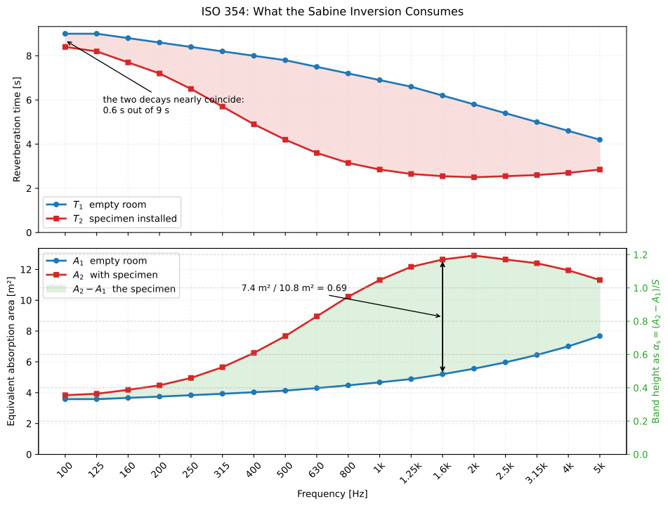
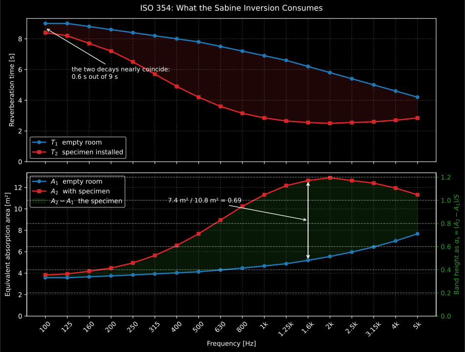
The whole ISO 354 inversion of the section 1 example, drawn: the two decay times (top) and the two Sabine areas they invert to (bottom), with the filled difference divided by m² giving the on the right-hand axis. At 100 Hz the two decays differ by 0.6 s out of 9 s and the filled band is barely visible, which is exactly why the uncertainty of section 4 is worst there. By 1.6 kHz the specimen has more than halved the decay and the difference is unmistakable.
Show the code for this figure
import matplotlib.pyplot as plt
# `meas` is the SoundAbsorptionMeasurement of section 1; every quantity the# figure draws is a field of it.fig, (ax_t, ax_a) = plt.subplots(2, 1, sharex=True, figsize=(10, 7))band = np.arange(freqs.size)ax_t.plot(band, meas.t_empty, "o-", label="T1 (empty room)")ax_t.plot(band, meas.t_specimen, "s-", label="T2 (specimen installed)")ax_t.set_ylabel("Reverberation time [s]")ax_t.legend()
a1 = meas.absorption_area_emptya2 = meas.absorption_area_with_specimenax_a.plot(band, a1, "o-", label="A1 (empty room)")ax_a.plot(band, a2, "s-", label="A2 (with specimen)")ax_a.fill_between(band, a1, a2, alpha=0.25, label="A2 - A1")ax_a.set_ylabel("Equivalent absorption area [m$^2$]")ax_a.set_xticks(band)ax_a.set_xticklabels([f"{f:g}" if f < 1000 else f"{f/1000:g}k" for f in freqs],                     rotation=45)ax_a.set_xlabel("Frequency [Hz]")ax_a.legend()plt.show()
print(np.round((a2 - a1) / 10.8 - meas.alpha_s, 12).max())   # 0.0: same alpha_s
Each of those two numbers is read off a decay, and the clip below shows how one is read: the squared impulse response is integrated backwards from the tail, the Schroeder curve emerges, and the T20 and T30 regressions are fitted to a straight portion of it. That is the operation behind , and again behind (the clip shows a single room, not the pair, so it answers “where does one come from” and not “what does subtracting two of them cost”). The second question is the one that governs this measurement, and section 4 puts a number on it: because is a difference of two reciprocal decay times, its uncertainty is worst exactly where the two decays are most alike, at the low-frequency end.
The tail energy of the squared impulse response fills from the end while the backward integral advances toward t = 0, and the Schroeder decay curve emerges on a companion axis, ending with the T20 and T30 regression lines.
The tail energy of the squared impulse response fills from the end while the backward integral advances toward t = 0, and the Schroeder decay curve emerges on a companion axis, ending with the T20 and T30 regression lines.
A room volume below the 150 m³ minimum or a
sample area outside 10–12 m² raises an advisory AbsorptionWarning; the result
still returns.
absorption_area() / absorption_coefficient() parameters
Section titled “absorption_area() / absorption_coefficient() parameters”| Parameter | Type | Units | Range / default | Notes |
|---|---|---|---|---|
t60 / t1, t2 | 1D array | s | > 0 | Reverberation time(s); t1 empty, t2 with specimen |
volume | float | m³ | > 0 | Room volume (advisory below 150 m³) |
sample_area | float | m² | > 0 | Area the specimen covers (coefficient only) |
temperature_c / temperature1_c, temperature2_c | float | °C | default 20.0, 15–30 | Sets via Eq. (6); temperature2_c defaults to temperature1_c |
speed_of_sound (…1, …2) | float, optional | m/s | > 0 | Overrides the temperature-derived |
m (m1, m2) | float or 1D array | 1/m | ≥ 0, default 0 | Air power attenuation coefficient |
absorption_area() returns the equivalent absorption area (m²) with the
shape of t60; absorption_coefficient() returns ;
attenuation_from_alpha(alpha) converts an ISO 9613-1 (dB/m) to .
3. Weighted rating and absorption class (ISO 11654)
Section titled “3. Weighted rating and absorption class (ISO 11654)”The measurement of section 1 delivers the spectrum in one-third-octave bands. ISO 11654:1997 turns that spectrum into a single-number rating comparable across products.
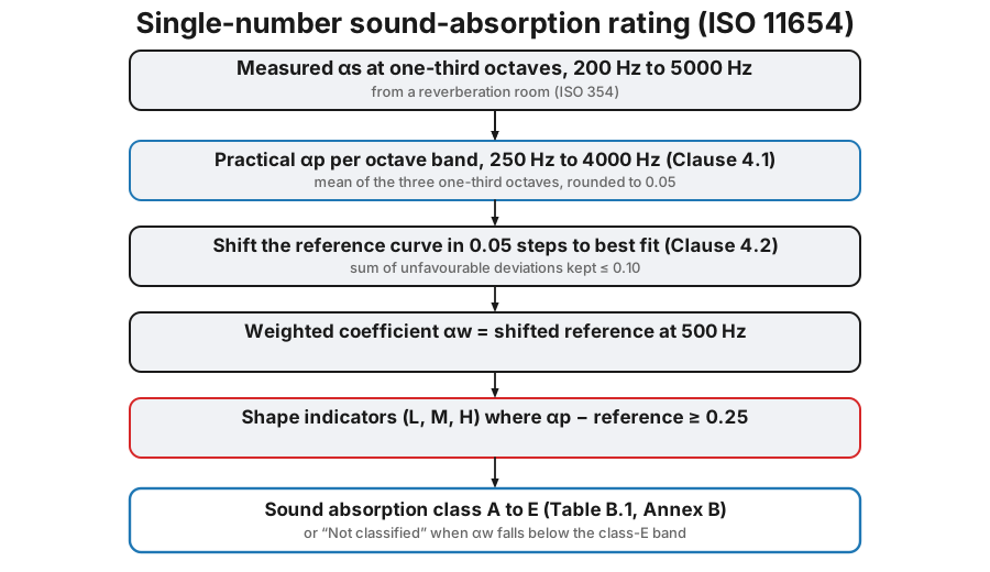
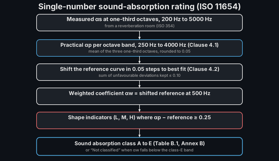
Practical absorption coefficient (Clause 4.1). The one-third-octave data are first grouped into octave bands, each the arithmetic mean of its three thirds:
evaluated to the second decimal and then rounded in steps of (the Clause 4.1 NOTE fixes the rounding, e.g. ); rounded means above are set to . The five rating bands are 250, 500, 1000, 2000 and 4000 Hz.
Weighted absorption (Clause 4.2). A fixed reference curve is shifted downwards, towards the measured , in steps of until the sum of the unfavourable deviations (taken only where the measurement lies below the shifted curve, with magnitude ) is no more than . The weighted coefficient is the shifted-curve value read at 500 Hz.
Shape indicators (Clause 4.3). When a practical coefficient exceeds the
shifted curve by or more, a shape indicator is appended: L at 250 Hz,
M at 500 or 1000 Hz, H at 2000 or 4000 Hz (e.g. 0.60(M)).
Absorption class (Table B.1). Finally maps to a class: A (0.90–1.00), B (0.80–0.85), C (0.60–0.75), D (0.30–0.55), E (0.15–0.25), or “not classified” (0.00–0.10). Because is always a multiple of these ranges partition the grid exactly.
What the rating cannot say. ISO 11654 scopes itself in Clause 1.2, and the
four limits it states there are exactly the cases a practitioner meets. The
reference curve starts at the 250 Hz octave, so everything the specimen does
at 100 Hz to 200 Hz is outside the rating by construction and the standard
says the rating “is not appropriate below this frequency”; a bass treatment
and a mid-frequency panel can share an while differing by half a
coefficient at 125 Hz. The rating is likewise “not applicable unless the
applications cover the whole frequency range of the reference curve”. If only
part of the range matters, the standard sends the reader back to the spectrum,
and points at the shape indicators as the hint that a modest with
an (L) may be the better product for a low-frequency problem. It is scoped
to routine applications (normal offices, corridors, classrooms, hospitals)
and declares itself inappropriate for “qualified environments requiring
careful acoustical design by expertise”, where only the full spectrum will do.
And it is “often not suitable for application to single items, such as chairs,
baffles, etc.” (whose absorption is an equivalent area per object, not a
coefficient), nor is it applicable to road barriers and road surfaces, which
have EN 1793-1 and
ISO 13472 of their own.
This is why the fiche always prints the whole spectrum beside the single
number.
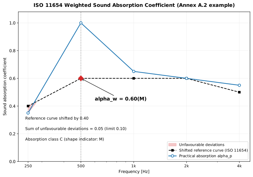
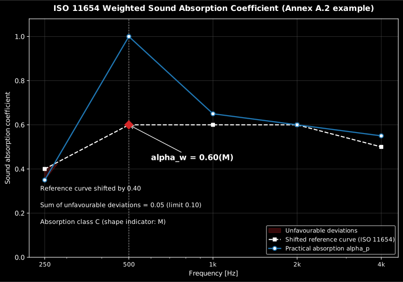
The Annex A.2 worked example: the reference curve is shifted down by 0.40 until
the unfavourable deviations sum to 0.05 (), giving ;
the 500 Hz peak overshoots the shifted curve by , adding the M
indicator, so the rating is , class C.
Show the code for this figure
import matplotlib.pyplot as pltfrom phonometry import materials
# ISO 11654 Annex A.2 practical coefficients at 250/500/1000/2000/4000 Hzresult = materials.weighted_absorption([0.35, 1.00, 0.65, 0.60, 0.55])result.plot()   # practical curve vs shifted reference, deviations shadedplt.show()
from phonometry import materials
# ISO 11654 Annex A.2 practical coefficients at 250/500/1000/2000/4000 Hzalpha_p = [0.35, 1.00, 0.65, 0.60, 0.55]
result = materials.weighted_absorption(alpha_p)print(result.rating_label) # 0.60(M)print(result.alpha_w) # 0.6print(result.absorption_class) # Cprint(round(result.unfavourable_sum, 2)) # 0.05result.plot() # the figure above: practical curve vs shifted reference
# A bare alpha_w also maps straight to its class (Table B.1)print(materials.absorption_class(0.85)) # Bweighted_absorption accepts the five octave-band values (as a
sequence or a {frequency: value} mapping); pass the fifteen one-third-octave
values to practical_absorption_coefficient first if you are starting
from raw ISO 354 data. To keep the one-third-octave on the result (so
the fiche can print the full table every accredited ISO 354 certificate carries),
rate it in one step with weighted_absorption_from_third_octave(alpha_s), which
forms , rates it and retains the input and its band centres
(third_octave_alpha_s, third_octave_bands). The result carries the shifted
reference curve and the per-band deviations, and its .plot() renders the figure
above.
from phonometry import materials
# Fifteen one-third-octave alpha_s (200 Hz to 5000 Hz), as an ISO 354 report givesalpha_s = [0.30, 0.35, 0.40, 1.00, 1.00, 1.00, 0.62, 0.66, 0.67,           0.58, 0.60, 0.62, 0.53, 0.55, 0.57]result = materials.weighted_absorption_from_third_octave(alpha_s)print(result.rating_label)          # 0.60(M)print(result.third_octave_alpha_s)  # the input alpha_s, retained for the fiche
Is that a good number? Absorption tracks thickness against wavelength, so every halving of the useful frequency costs a doubling of thickness or of cavity depth, and the ladder is short. Predicting a mineral-wool-class material ( kPa·s/m²) hard against a wall with the multilayer models gives a random-incidence coefficient at 500 Hz of about 0.32 for a 25 mm blanket, 0.68 for 50 mm and 0.89 for 100 mm; at 250 Hz the same three give 0.14, 0.37 and 0.74. Spacing the 50 mm layer off the wall on a 100 mm cavity lifts its 250 Hz value from 0.37 to 0.68: the cavity buys roughly the octave that doubling the material would have bought. A painted or sealed hard surface sits at a few hundredths across the whole range. The practical reading: class A is nearly always a thick or a spaced construction rather than a clever surface, and a thin sample that reports a mid-frequency above about 1.1, or a rising low-frequency tail, is showing an edge effect or a mounting leak rather than a good material. Measured ISO 354 values also run above these predicted ones, by roughly 0.1 to 0.2 in the mid bands, for the finite-sample reason set out in the closing section.
ISO 11654 report (.report())
Section titled “ISO 11654 report (.report())”AbsorptionRatingResult.report(path) renders a one-page PDF fiche laid out like
an accredited absorption test report (an ISO 354 reverberation-room measurement
rated per ISO 11654): a standard-basis line, an optional metadata header block,
the octave-band table beside the practical-versus-shifted-reference
plot (the result’s own .plot()), the boxed single number with its
absorption class and applied shift, an optional verdict row and a footer with
the fixed disclaimer. When the rating was built with
weighted_absorption_from_third_octave, the left table becomes the full ISO 354
one-third-octave table with the octave on the matching
rows, exactly as accredited certificates print it. It uses the same
ReportMetadata container and rendering engine as the
ISO 717 insulation fiche;
passing metadata=None produces a lightweight prediction fiche, and a supplied
requirement is read as the minimum for the PASS/FAIL verdict.
Setting verbose=True swaps the two-column table for the ISO 11654 evaluation
columns (practical coefficient, shifted reference, unfavourable deviation).
Rendering needs reportlab and, for the figure the fiche embeds, matplotlib (pip install "phonometry[report,plot]"); only engine="reportlab" is supported. The
fiche renders in English by default; pass language="es" for a Spanish fiche
(translated fixed strings and a comma decimal separator), e.g.
result.report("alpha_w_fiche_es.pdf", language="es").
from phonometry import materials, ReportMetadata
# Rate from the fifteen one-third-octave alpha_s so the fiche prints the full# ISO 354 table; materials.weighted_absorption([...]) also works from alpha_p.alpha_s = [0.30, 0.35, 0.40, 1.00, 1.00, 1.00, 0.62, 0.66, 0.67,           0.58, 0.60, 0.62, 0.53, 0.55, 0.57]result = materials.weighted_absorption_from_third_octave(alpha_s)result.report(    "alpha_w_fiche.pdf",    metadata=ReportMetadata(        specimen="50 mm porous absorber over a 100 mm air gap",        area=10.8, mounting="Type A (against a rigid wall)",        measurement_standard="ISO 354",        temperature_c=21.4, relative_humidity_percent=54.0,        laboratory="Phonometry Reference Laboratory",        requirement=0.55,          # adds the PASS/FAIL verdict row    ),)                                  # alpha_w (shape) + absorption class
The example fiche is regenerated with make reports and kept rendered in the
repository; click the preview to open the PDF.
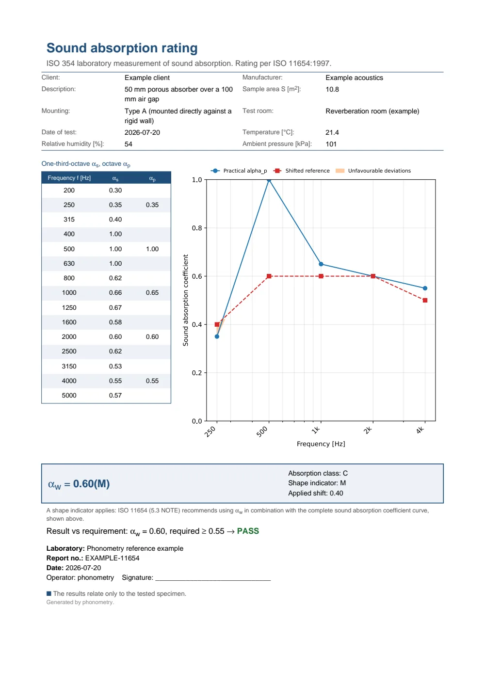
One-page sound absorption fiche: a metadata header (client, specimen, sample area, mounting, reverberation-room temperature, humidity and pressure), the full one-third-octave alpha_s table with the octave alpha_p on the matching rows beside the practical-versus-shifted-reference plot, the boxed alpha_w = 0.60 (M) single-number result with absorption class C and the applied shift, and a PASS verdict against the 0.55 requirement.
4. Sound-absorption measurement uncertainty (ISO 12999-2)
Section titled “4. Sound-absorption measurement uncertainty (ISO 12999-2)”A rated absorption coefficient means little without its uncertainty. ISO 12999-2:2020 gives the standard uncertainty of the quantities produced by a reverberation-room measurement (ISO 354) and its ratings (ISO 11654, EN 1793-1), estimated from inter-laboratory tests to ISO 5725. It is the sound-absorption companion of the sound-insulation uncertainty of ISO 12999-1 (Field Insulation Measurement (ISO 16283)).
One-third-octave bands (Clause 5). For the sound-absorption coefficient the reproducibility standard deviation is (Formula (1)), and for the equivalent absorption area with (Formula (2)), where and are the frequency-dependent regression constants of Table 1 (63–5000 Hz): nothing to do with the air power attenuation coefficient of section 1, which shares the standards’ letter and not its meaning. The repeatability value is (Formula (3)). Note that the term of Formula (2) is multiplied by a fixed reference area of 10 m² rather than by the specimen’s own area, so a small specimen’s is proportionally far less certain than a large one’s (which is one more reason ISO 354 pins the test area between 10 m² and 12 m²).
Practical coefficient (Clause 6). For the ISO 11654 practical coefficient
in octave bands with the constants of Table 2
(250–4000 Hz); again . Table 2 covers those five
octaves only, so the 125 Hz octave has no tabulated uncertainty and
practical_coefficient_uncertainty rejects it rather than returning a blank.
Single numbers (Clause 7). The weighted coefficient has a constant standard uncertainty (, ); the EN 1793-1 single-number rating scales with the value (, ).
Reporting (Clause 8). The expanded uncertainty is (Formula (10))
with the Table 3 coverage factor ( at 95 %, Gaussian; read another
confidence off the same table with absorption_coverage_factor, which returns
2.6 at 99 %). The reported is rounded to two decimals for absorption
coefficients and one decimal for the equivalent area and
.
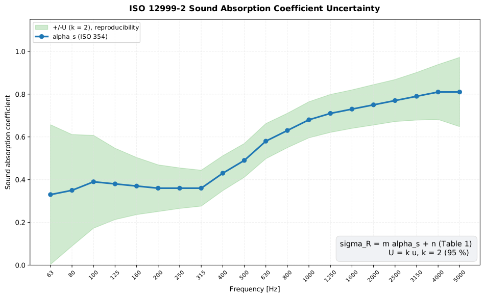
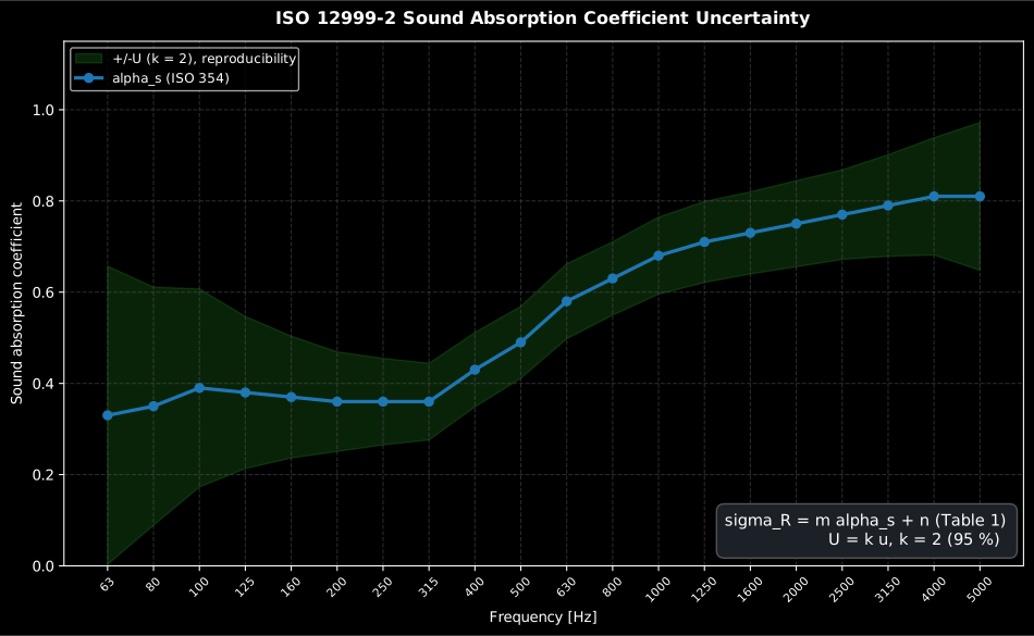
The Table 4 worked example: the measured spectrum with its ribbon at (95 %), where takes and from Table 1. The ribbon is a shallow U: in the 63 Hz band, tightening to from 250 Hz to 2 kHz and opening again to at 5 kHz. The width is set almost entirely by the band, not by the absorber: the low end is the modal field of the room, the high end is the air absorption the two decays must be corrected for. The plotted is the reported one, rounded to two decimals as Clause 8 requires.
Show the code for this figure
import matplotlib.pyplot as pltfrom phonometry import materials
# ISO 12999-2 Table 4 worked example: alpha_s per one-third-octave band.freqs = [63, 80, 100, 125, 160, 200, 250, 315, 400, 500,         630, 800, 1000, 1250, 1600, 2000, 2500, 3150, 4000, 5000]alpha_s = [0.33, 0.35, 0.39, 0.38, 0.37, 0.36, 0.36, 0.36, 0.43, 0.49,           0.58, 0.63, 0.68, 0.71, 0.73, 0.75, 0.77, 0.79, 0.81, 0.81]result = materials.sound_absorption_coefficient_uncertainty(alpha_s, freqs, confidence=0.95)result.plot()   # alpha_s with the +/-U (k = 2) reproducibility ribbonplt.show()
from phonometry import materials
# Reproducibility uncertainty of alpha_s at 1000 Hz (Table 1: m=0.040, n=0.015).r = materials.sound_absorption_coefficient_uncertainty([0.68], [1000], confidence=0.95)print(round(float(r.standard_uncertainty[0]), 4)) # 0.0422 (sigma_R)print(float(r.reported_expanded_uncertainty[0])) # 0.08 (U, k=2)r.plot() # the figure above: alpha_s with its +/-U (k = 2) ribbon
# Same band, same value, but a repeat on my own bench rather than another# laboratory: sigma_r = 0.6 sigma_R (Formula (3)).rr = materials.sound_absorption_coefficient_uncertainty( [0.68], [1000], condition="repeatability")print(round(float(rr.standard_uncertainty[0]), 5)) # 0.02532 = 0.6 x 0.0422
# The other two quantities this page produces, Formula (2) and Clause 6.at = materials.equivalent_area_uncertainty([12.4], [1000], confidence=0.95)print(float(at.reported_expanded_uncertainty[0])) # 1.3 m^2 on A_T = 12.4 m^2ap = materials.practical_coefficient_uncertainty( [0.35, 1.00, 0.65, 0.60, 0.55], [250, 500, 1000, 2000, 4000])print(list(ap.reported_expanded_uncertainty)) # [0.07, 0.08, 0.08, 0.08, 0.1]
# Single-number ratings (Clause 7 worked examples).print(float(materials.weighted_coefficient_uncertainty(0.70).reported_expanded_uncertainty[0])) # 0.07print(float(materials.single_number_rating_uncertainty(8.1).reported_expanded_uncertainty[0])) # 1.6What those numbers mean. An expanded uncertainty of 0.08 on a one-third-octave is a statement about two laboratories: measuring the same product, both correctly, they may legitimately report 0.64 and 0.72, so a specification written to two decimals is not testable and a datasheet value that misses your own measurement by less than the combined is agreement, not a discrepancy. Within one laboratory the repeatability figure applies instead: 0.6 of the reproducibility value, a spread about 40 % narrower. So a repeat on your own bench that falls outside the narrower band points at the specimen, the mounting or the room, not at the method. The single numbers are worse than they look: exceeds the 0.05 step is quoted on, so a product measured at 0.85 (class B) cannot be told apart from one at 0.90 (class A) by a single test. A tender that hinges on a class letter is a tender decided by measurement noise; ask for the spectrum and the uncertainty instead, and quote beside in the fiche.
Tube or reverberation room?
Section titled “Tube or reverberation room?”The tube and the reverberation room both deliver a number called the “absorption coefficient”, and the two are routinely confused. They are different physical quantities, measured under different sound fields, and they do not match, sometimes not even closely.
The tube measures a normal-incidence coefficient: one plane wave, one angle, a specimen a few centimetres across, and a complex reflection factor that keeps magnitude and phase. ISO 354 measures the random-incidence coefficient : a diffuse field striking a sample of 10 m² to 12 m² from every direction at once, recovered from the change in the room’s decay time through Sabine’s formula, an energy average with no phase left in it. Because the diffuse field finds more ways into an absorber than the single normal-incidence wave (oblique waves travel a longer path inside the layer), usually comes out higher. For a locally reacting surface the two are linked by Paris’ angular average, which defines the statistical absorption coefficient
an integral that weights the oblique angles most heavily. It needs the
angle-dependent , not the normal-incidence coefficient itself.
But for a locally reacting surface follows from the
normalised surface impedance alone, so the integral has a closed form and a
tube result converts in one line:
materials.statistical_absorption(result.normalized_impedance), documented
with the
multilayer models.
What that cannot do is cover a bulk-reacting layer, where the oblique
behaviour depends on refraction inside the material and the integral has to be
evaluated angle by angle from a model: diffuse_field_absorption, on the same
page.
The size of the gap is worth seeing, because “usually higher” is not a useful design statement:
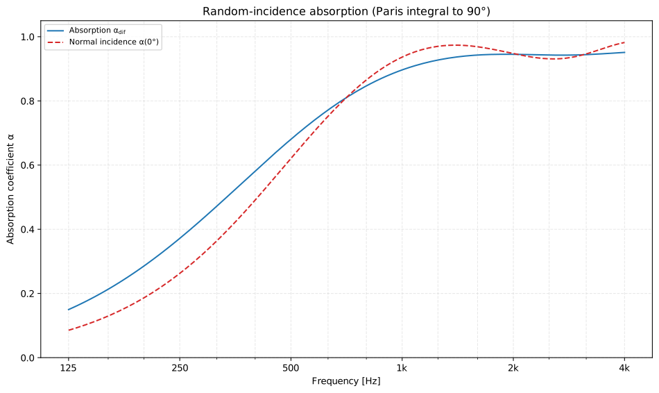
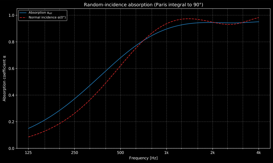
What the tube reads and what the room reads, for the same 50 mm hard-backed porous layer ( kPa·s/m², Miki): the tube measures , the dashed curve, while the room measures the Paris average over all angles, the solid one. The gap is widest where the layer is thin against the wavelength: precisely the low-frequency region where a normal-incidence number substituted into a Sabine or EN 12354-6 budget would underpredict the installed absorption, and closes as the layer becomes electrically thick. It is a model comparison on an infinite layer, so it is a lower bound on the real difference: a finite ISO 354 specimen adds the edge effect on top.
Show the code for this figure
import matplotlib.pyplot as plt
# A 50 mm porous layer on a rigid backing, predicted both ways.f = np.geomspace(125.0, 4000.0, 200)layers = [materials.PorousLayer(0.05, materials.miki(f, 20000.0))]normal = materials.layered_absorber(f, layers)diffuse = materials.diffuse_field_absorption(f, layers)ax = diffuse.plot()ax.plot(f, normal.absorption, ls="--", label="Normal incidence")ax.legend()plt.show()
Why ISO 354 values exceed 1. A ratio of absorbed to incident energy cannot exceed one, yet reverberation-room reports of to for thick porous absorbers are routine and correct by the method. Sabine’s formula converts the decay-time change into an equivalent absorption area , and divides by the geometric sample area . Diffraction at the sample edges lets the specimen drain energy from a sound field wider than its footprint (the edge effect), so the equivalent area can exceed the geometric one. Such values are not errors, but they are not portable either: they depend on the sample size and perimeter, which is precisely why ISO 354 fixes both. The ISO 11654 rating simply truncates: practical coefficients above are set to (section 3). Prediction inputs get no such silent clipping in this library: each reverberation-time estimator enforces its own mathematical domain, so Sabine and Eyring accept ISO 354 values at or above one as supplied (Eyring as long as the mean absorption stays below one), while Millington-Sette rejects them (its per-surface logarithm diverges at one) and any adjustment below one is left to the caller. The equivalent-absorption-area budget of EN 12354-6 likewise accepts the coefficients as supplied.
Which to use. They answer different questions. The reverberation-room value is the one that feeds diffuse-field prediction: Sabine reverberation estimates, the equivalent absorption areas of EN 12354-6 and the rating and class, all of which expect random incidence over a mounted, finite sample (ISO 354’s Annex B mounting types exist because the mounting is part of the result). The tube value is the laboratory and development tool: it needs only a few square centimetres of material, resolves magnitude and phase, and its surface impedance pins down the parameters of porous-material models in the Allard and Atalla tradition, with the airflow resistivity as the first input; the fitted model then predicts the layer at any angle, thickness or backing. What the tube number is not is a drop-in substitute for : feeding normal-incidence coefficients into a Sabine or EN 12354-6 budget systematically underpredicts the installed absorption.
What this guide covers
Section titled “What this guide covers”Covered
The ISO 354:2003 Sabine inversion (Eqs. (5)-(9)) in
measure_sound_absorption, and the Clause 4/8.1 conversion of an already-measured / pair inabsorption_areaandabsorption_coefficient(withattenuation_from_alphafor the air term). ISO 11654:1997’s weighted absorption rating: the practical coefficient of Clause 4.1, the reference-curve shift of Clause 4.2, the shape indicators of Clause 4.3, and the Table B.1 absorption class, built byweighted_absorptionandweighted_absorption_from_third_octave. ISO 12999-2:2020’s measurement-uncertainty formulae (Clauses 5-8), one function per quantity:sound_absorption_coefficient_uncertainty(Formula (1)),equivalent_area_uncertainty(Formula (2)),practical_coefficient_uncertainty(Clause 6),weighted_coefficient_uncertaintyandsingle_number_rating_uncertainty(Clause 7), each takingcondition="reproducibility"or"repeatability"for Formula (3), with the Table 3 coverage factor inabsorption_coverage_factor.Not covered
Nothing on this page consumes a measured surface impedance: the conversion from a tube result to the statistical coefficient lives with the prediction models (
statistical_absorptionfor a locally reacting surface,diffuse_field_absorptionfor a bulk-reacting one), and neither is a substitute for an ISO 354 measurement, because neither reproduces the edge effect. The room and specimen requirements of Clause 6 and Annex A are described in sections 1.2 and 1.3 but not checked: nothing here verifies the shape rule, the Table 1 ceiling on , the diffusivity qualification or the microphone and source counts, andabsorption_area/absorption_coefficientonly convert an already-measured / pair and raise an advisory warning when the room volume or sample area falls outside the Clause 6 limits. Neither is the decay measurement itself in scope; the interrupted-noise and integrated-impulse-response methods of Clause 7 belong to room acoustics. ISO 12999-2’s uncertainty formula for the EN 1793-1 single-number rating is implemented, but EN 1793-1’s own in-situ measurement method (road-traffic noise-reducing devices) is not.
References
Section titled “References”- Cox, T. J., & D'Antonio, P. (2017). Acoustic absorbers and diffusers: Theory, design and application (3rd ed.). CRC Press. https://doi.org/10.1201/9781315369211Absorber measurement in practice: the room method, mountings, and the edge-effect discussion behind the tube-or-reverberation-room section. ISBN 978-1-4987-4099-9.
- International Organization for Standardization. (1997). Acoustics — Sound absorbers for use in buildings — Rating of sound absorption (ISO 11654:1997). The weighted sound-absorption rating of section 3: the practical coefficient, the shifted reference curve, the shape indicators and the absorption class, validated against the standard's own Annex A worked example.
- International Organization for Standardization. (2003). Acoustics — Measurement of sound absorption in a reverberation room (ISO 354:2003). The reverberation-room method of section 1 that produces the alpha_s spectra rated by ISO 11654, including the Annex B specimen mountings.
- International Organization for Standardization. (2020). Acoustics — Determination and application of measurement uncertainties in building acoustics — Part 2: Sound absorption (ISO 12999-2:2020). The sound-absorption measurement uncertainty of section 4, validated against the standard's own worked examples (Tables 4/5).