Metadiffusers
Key references: Jiménez et al. 2017Jiménez et al. 2019Cox & D'Antonio 2017Jiménez et al. 2016Jiménez et al. 2021
A Schroeder diffuser earns its diffusion with depth: the design equations turn a phase sequence into wells whose maximum depth approaches half the design wavelength, so a diffuser for the low hundreds of hertz is tens of centimetres thick, and that thickness is what keeps phase-grating diffusers out of small rooms, studios and vehicles. A metadiffuser (Jiménez, Cox, Romero-García and Groby, 2017) reaches the same reflection phases from a panel one to two orders of magnitude thinner: each well becomes a thin closed slit loaded by Helmholtz resonators, and the resonators slow the sound inside the slit so drastically that a 2 cm panel behaves like wells 27 cm deep. This guide covers the slow-sound mechanism, the published quadratic-residue metadiffuser evaluated end to end, and the design recipe that maps any Schroeder sequence onto a deep-subwavelength panel.
1. Slow sound in a loaded slit
Section titled “1. Slow sound in a loaded slit”The unit cell is the same one the slow-sound absorber is built from: a slit of height runs the depth of the panel and is loaded, along its upper wall, by an array of Helmholtz resonators on a lattice step . The slit chain is evaluated with the transfer-matrix method,
half-lattice slit steps around each resonator, the resonators as shunt point scatterers , and a slit-radiation end correction , with visco-thermal effective parameters in the slit and in the square necks and cavities (Stinson 1991). Below the resonance of the loading resonators the shunt compliance adds to the compliance of the slit itself, and the effective phase velocity of the slit mode collapses: the retrieved effective wavenumber of the chain corresponds to a phase speed of a few tens of metres per second. The slit therefore reaches its quarter-wavelength condition, and any intermediate reflection phase, at a fraction of the depth an air-filled well would need.
Two consequences make the mechanism ideal for diffusers rather than just absorbers:
- The reflection phase is tunable per slit. The rigidly backed slit reflects with , and the resonator geometry tunes the phase of through the full range at the working frequency while stays close to one. A phase profile that a classical grating writes with depth, the metadiffuser writes with resonator tuning.
- Critical coupling adds a third state. Driving one slit to critical coupling balances its visco-thermal loss against its leakage and produces a reflection zero: . Ternary sequences (reflection values , , ) need exactly that perfectly absorbing state, which no rigid well can provide.
metadiffuser_reflection runs that chain once per well (two-dimensional
resonators, visco-thermal losses and end corrections included) and returns the
per-well complex reflection ; metadiffuser_polar_response and
metadiffuser_diffusion_spectrum reduce that spatial profile through the same
Fraunhofer far field and ISO 17497-2 coefficient used for the
classical designs. A None entry in the well
sequence stands for a flat rigid strip (), the state of ternary
designs.
2. The published quadratic-residue metadiffuser
Section titled “2. The published quadratic-residue metadiffuser”The published design packs a whole quadratic-residue diffuser into a
35 cm x 2 cm panel: five slits, each loaded by two resonators, on a 7 cm
pitch. This is a quadratic-residue design, so all five slits are meant to
reflect with near one and to differ only in phase. Two of them, slits 1
and 4, do come close to critical coupling (their absorption peaks at 0.99)
but at 2305 Hz and 2260 Hz, above the 2 kHz the phase profile is tuned for,
where they still reflect 0.97 of the incident pressure. The critically coupled
slit that a
ternary sequence needs as its 0 state is the same kind of cell driven
deliberately onto resonance at the working frequency, which is what
critical_coupling_design
solves for. This published panel is the QRD case, and at 2 kHz it scatters
like the 27.4 cm deep diffuser it mimics.
As in the published far-field comparison, the polar response repeats the
five-well sequence six times (repetitions=6, a 2.1 m panel):
import numpy as npfrom phonometry import materials
# The published quadratic-residue metadiffuser: five slits with two# resonators each in a 35 cm x 2 cm panel (7 cm pitch), tuned to mimic a# QRD designed for 500 Hz whose wells would run up to 27.4 cm deep.mm = 1e-3# The row order follows the published table; HelmholtzResonator takes# (neck_length, neck_side, cavity_length, cavity_side), hence the reshuffle.rows = [  # slit h, neck l_n, cavity l_c, neck w_n, cavity w_c  [mm]    (14.7, 13.0, 16.4, 6.2, 9.0),    (30.9, 9.1, 4.3, 3.5, 9.0),    (30.9, 9.1, 4.3, 3.5, 9.0),    (15.7, 13.3, 17.0, 6.3, 9.0),    (20.3, 18.0, 20.7, 3.2, 9.0),]wells = []for h, ln, lc, wn, wc in rows:    resonator = materials.HelmholtzResonator(ln * mm, wn * mm, lc * mm, wc * mm)    # two identical resonators per slit    wells.append(materials.MetadiffuserWell(h * mm, (resonator, resonator)))
f = np.arange(1800.0, 2601.0, 5.0)panel = materials.metadiffuser_reflection(f, wells, depth=0.02, period_m=0.07)alpha1 = panel.well_absorption[0]print(round(float(alpha1.max()), 2), int(f[alpha1.argmax()]))  # 0.99 2305
# What the panel absorbs where it is used, not where it resonates.i2k = int(np.argmin(np.abs(f - 2000.0)))print(np.round(panel.well_absorption[:, i2k], 3))# [0.054 0.009 0.009 0.055 0.032]print(round(float(panel.absorption[i2k]), 3))       # 0.032peak = int(f[panel.absorption.argmax()])print(round(float(panel.absorption.max()), 3), peak)# 0.253 2260
# Far-field comparison: the five-well sequence repeated six times (2.1 m).polar = materials.metadiffuser_polar_response(2000.0, wells, depth=0.02,                                              period_m=0.07, repetitions=6)print(round(polar.coefficient, 2))                             # 0.32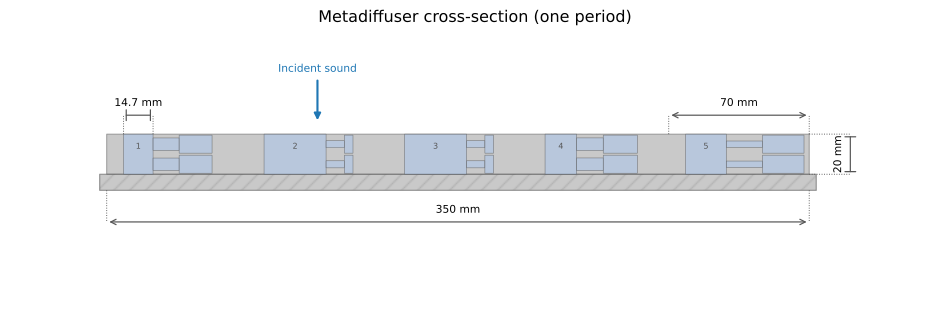
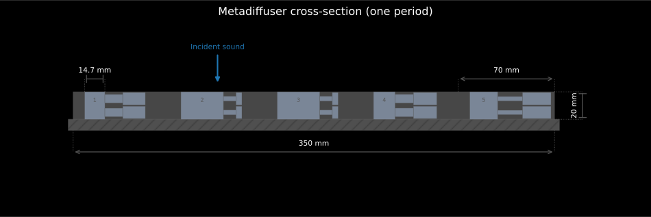
One period to scale: five slits from 14.7 mm to 30.9 mm tall on a 70 mm pitch inside a 350 mm × 20 mm panel, each loaded by two Helmholtz resonators shelved sideways into the septum that separates it from its neighbour. The whole panel is 20 mm deep against the 686 mm wavelength of its 500 Hz reference design, one part in 34.
Show the code for this figure
import matplotlib.pyplot as plt
# `panel` is the MetadiffuserResult computed above, and it retains the# geometry it was computed for, so it redraws its own cross-section:panel.plot_geometry()plt.show()
# From a bare well list, without computing a reflection first, the same# drawing comes from materials.plot_metadiffuser_panel_geometry(#     wells, depth=0.02, period_m=0.07).
At the 2 kHz design frequency the panel is essentially a phase grating: it
reflects 96.8 % of the incident energy and absorbs 3.2 %, per slit no more
than 5.5 %. Three hundred hertz higher it is a different surface. Slits 1 and
4 pass through critical coupling at 2305 Hz and 2260 Hz with absorption
coefficients of 0.99, so two fifths of the panel area briefly becomes a
near-perfect absorber and the face average reaches 0.25. .plot() on the
result draws exactly that.
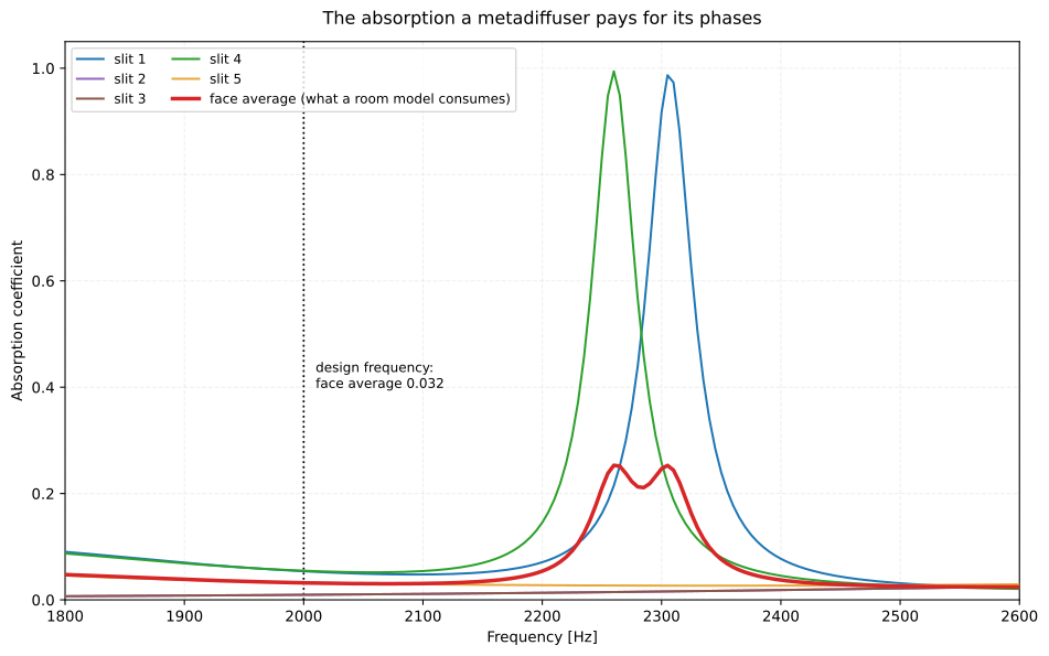
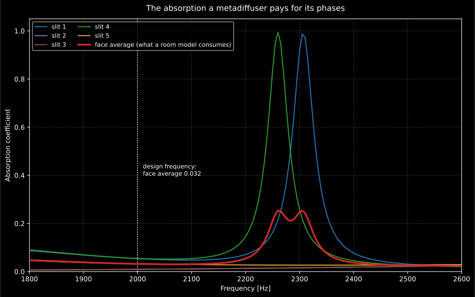
A metadiffuser is not lossless, and the loss is not flat. At the design frequency the face average is 0.03, which a room model can usually ignore beside the diffusion coefficient; between the two critical-coupling peaks it is 0.25, which it cannot. The panel doubles as a narrow-band absorber at 2.3 kHz whether or not that was wanted, and the absorption spectrum belongs on the datasheet next to the diffusion spectrum.
Show the code for this figure
import matplotlib.pyplot as plt
# `panel` is the MetadiffuserResult computed above. One line:panel.plot()plt.show()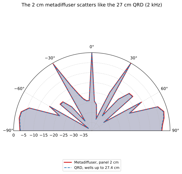
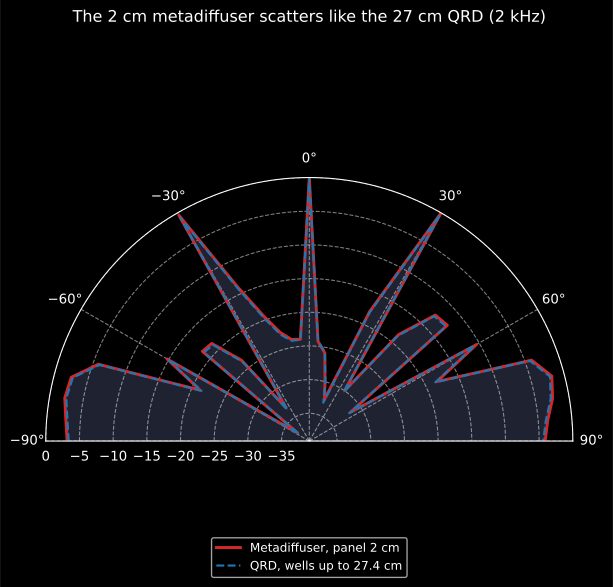
The claim of the whole guide, in one overlay: the same grating lobes in the same directions at the same levels, from a panel 13.7 times thinner. Both responses are six periods of the five-well sequence, a 2.1 m array, so the only difference between them is how each well reaches its reflection phase.
Show the code for this figure
import numpy as npfrom phonometry import materials
mm = 1e-3rows = [    (14.7, 13.0, 16.4, 6.2, 9.0),    (30.9, 9.1, 4.3, 3.5, 9.0),    (30.9, 9.1, 4.3, 3.5, 9.0),    (15.7, 13.3, 17.0, 6.3, 9.0),    (20.3, 18.0, 20.7, 3.2, 9.0),]wells = [    materials.MetadiffuserWell(        h * mm,        2 * (materials.HelmholtzResonator(ln * mm, wn * mm, lc * mm, wc * mm),),    )    for h, ln, lc, wn, wc in rows]
# The metadiffuser panel and the QRD it was tuned to at 2 kHz, both with# six repetitions of the period_m (2.1 m panels).meta = materials.metadiffuser_polar_response(2000.0, wells, depth=0.02, period_m=0.07,                                             repetitions=6)sequence = np.roll(materials.quadratic_residue_sequence(5), -1)depths = sequence * (343.0 / 500.0) / (2 * 5)qrd = materials.predict_diffuser_polar_response(    0.07, 2000.0, depths=depths, repetitions=6, include_obliquity=False,)
ax = meta.plot(marker="", linewidth=2.2, label="Metadiffuser, panel 2 cm")qrd.plot(ax=ax, marker="", linewidth=1.6, linestyle="--",         label="QRD, wells up to 27.4 cm")ax.legend(loc="lower center")
The far-field overlay above is the frequency-domain summary; the FDTD animation below meshes both panels for real (the metadiffuser at 0.25 mm, slits, necks and cavities included) and lets the same 2 kHz wavefront hit them: the 27 cm QRD and the 2 cm panel throw out nearly the same scattered fan.
A 2 kHz plane wavefront hits a Schroeder diffuser with wells down to 27 centimetres and, beside it, the 2 centimetre metadiffuser of the published design, whose real slits, necks and cavities are meshed at 0.25 millimetres. The total field and the persistent scattered envelope show both panels spraying nearly identical diffuse fans, and the receiver-arc diffusion coefficients confirm it quantitatively.
A 2 kHz plane wavefront hits a Schroeder diffuser with wells down to 27 centimetres and, beside it, the 2 centimetre metadiffuser of the published design, whose real slits, necks and cavities are meshed at 0.25 millimetres. The total field and the persistent scattered envelope show both panels spraying nearly identical diffuse fans, and the receiver-arc diffusion coefficients confirm it quantitatively.
3. The design recipe: phases first, geometry second
Section titled “3. The design recipe: phases first, geometry second”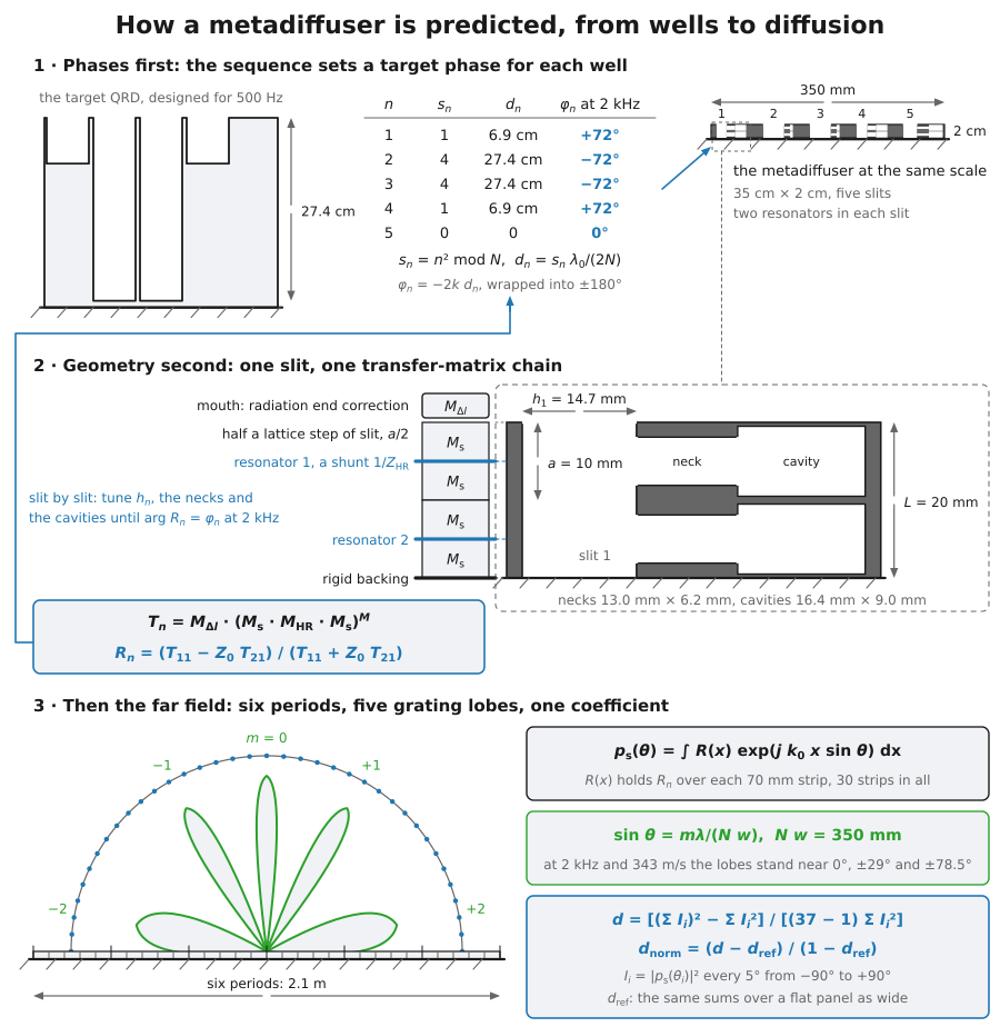
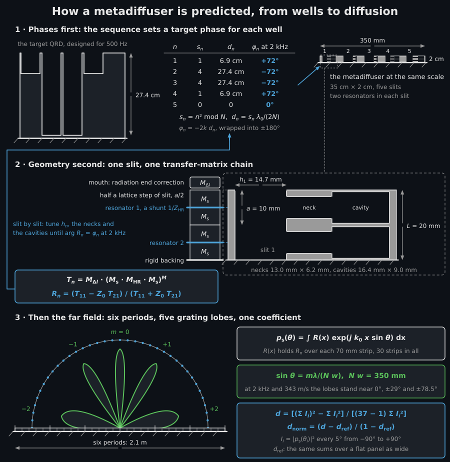
The whole prediction in one figure, for the published panel. The quadratic residues fix one phase per well; each slit is then tuned, through the transfer-matrix chain, until it returns that phase from 20 mm of depth; and only then do six periods go through the far field to a diffusion coefficient. The two panels at the top share one scale: 27.4 cm of wells against 2 cm of slits.
Designing a metadiffuser is a two-step translation. First pick the Schroeder
sequence exactly as for a classical design:
the quadratic residues give the target well depths
and hence the target reflection phases
at the evaluation frequency. Second, tune each slit
(its height, and the neck and cavity of its resonators) until the chain
reproduces that phase from the fixed panel depth . The per-well reflection
returned by metadiffuser_reflection is the quantity to match; for the
published design at 2 kHz the five slits land within a few degrees of the QRD
targets while keeping near one:
import numpy as npfrom phonometry import materials
# wells: the five published slits from the example above.panel = materials.metadiffuser_reflection(np.array([2000.0]), wells,                                          depth=0.02, period_m=0.07)phases = np.degrees(np.angle(panel.reflection[:, 0]))print(np.round(np.abs(panel.reflection[:, 0]), 2))  # [0.97 1.   1.   0.97 0.98]print(np.round(phases))                             # [ 75. -71. -71.  74.   2.]
# The targets: the 500 Hz N = 5 QRD it mimics, evaluated at 2 kHz.sequence = np.roll(materials.quadratic_residue_sequence(5), -1)depths = sequence * (343.0 / 500.0) / (2 * 5)          # up to 27.4 cm deepk = 2 * np.pi * 2000.0 / 343.0targets = np.degrees(np.angle(np.exp(-2j * k * depths)))print(np.round(targets))                            # [ 72. -72. -72.  72.   0.]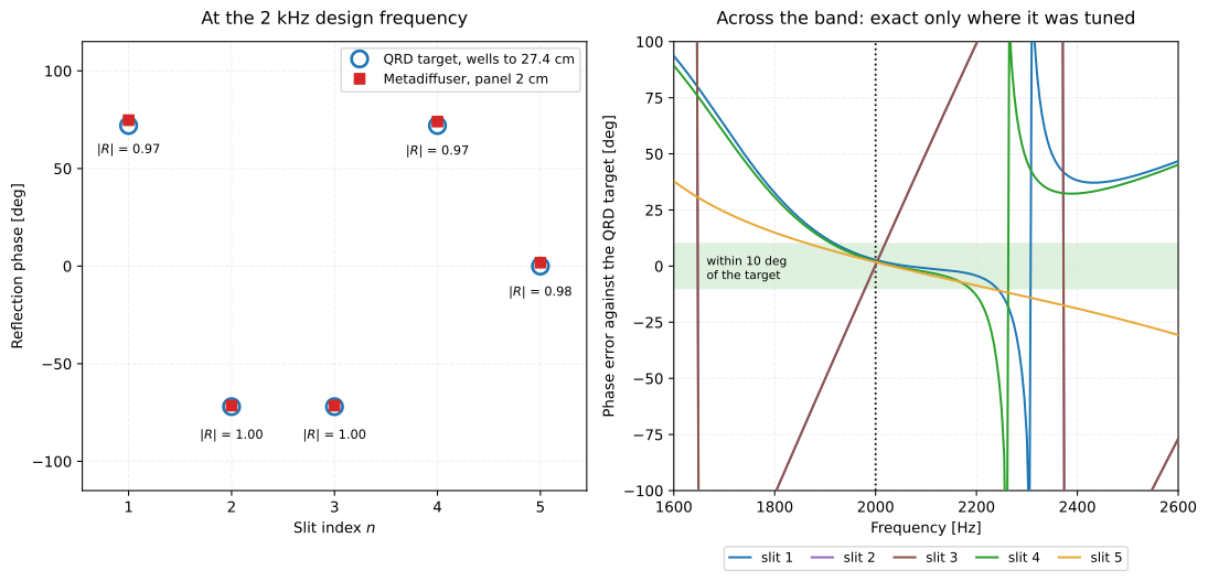
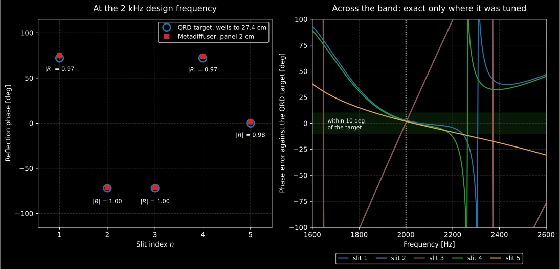
Left: the whole trick. Five slits 20 mm deep land on the phases of wells up to 27.4 cm deep, within 3°, while still reflecting 0.97 to 1.00 of the incident pressure. Right: the limit of the trick. The rigid well’s phase is linear in frequency and the loaded slit’s is not, so the match is exact only where it was driven to zero. Slits 2 and 3 have identical geometry and their curves coincide; slit 5, the zero-depth member of the sequence, is the only one that stays within 10° over more than a few hundred hertz.
Show the code for this figure
import matplotlib.pyplot as plt
# `wells` and `depths` come from the blocks above.sweep = np.linspace(1600.0, 2600.0, 201)swept = materials.metadiffuser_reflection(sweep, wells, depth=0.02, period_m=0.07)k_sweep = 2 * np.pi * sweep / 343.0target_phase = np.angle(np.exp(-2j * np.outer(depths, k_sweep)))error = np.degrees(np.angle(np.exp(1j * (np.angle(swept.reflection)                                         - target_phase))))fig, ax = plt.subplots()ax.axhspan(-10.0, 10.0, color="#2ca02c", alpha=0.15)labels = ("slit 1", "slit 2", "slit 3", "slit 4", "slit 5")for row, label in zip(error, labels):    ax.plot(sweep, row, label=label)ax.set_ylim(-100.0, 100.0)ax.set_xlabel("Frequency [Hz]")ax.set_ylabel("Phase error against the QRD target [deg]")ax.legend()plt.show()
Step two, worked. The paragraph above says “tune each slit until the chain
reproduces that phase”, which is a search, not a formula, and the page owes
the reader one. The parameter space of a slit is four numbers: its height,
and the neck length, neck side and cavity length of its resonators, and
metadiffuser_reflection on one panel is cheap, so the search is a loop. The
panel depth is fixed by the application before anything else is chosen;
after that the cavity length is the coarse control on the resonance and hence
on the phase, the neck is the fine control, and the slit height is the coarse
control on how much loss the slit carries. Sweeping the one coarse parameter
recovers the published cavity length to within a grid step:
import numpy as np
# `rows`, `wells` and `targets` come from the blocks above. Rebuild the panel# with a candidate cavity length in slit 1 and keep the geometry that lands# nearest its target phase while still reflecting almost everything.def panel_with(cavity_mm):    trial = [(14.7, 13.0, cavity_mm, 6.2, 9.0)] + rows[1:]    built = []    for h, ln, lc, wn, wc in trial:        resonator = materials.HelmholtzResonator(ln * mm, wn * mm, lc * mm, wc * mm)        built.append(materials.MetadiffuserWell(h * mm, (resonator, resonator)))    return materials.metadiffuser_reflection(np.array([2000.0]), built,                                             depth=0.02, period_m=0.07)
best = Nonefor cavity_mm in np.linspace(4.0, 22.0, 60):    r1 = complex(panel_with(cavity_mm).reflection[0, 0])    if abs(r1) < 0.9:            # the designer's own floor on |R_n|        continue    err = abs(np.degrees(np.angle(np.exp(        1j * (np.angle(r1) - np.radians(targets[0]))))))    if best is None or err < best[1]:        best = (cavity_mm, err)print(round(best[0], 2), round(best[1], 1))   # 16.81 1.1# The published table gives 16.4 mm for this slit: one grid step away.
Five such loops, one per slit, are the whole inverse problem. The library leaves them explicit rather than wrapping them because the cost function is the designer’s: how much phase error is acceptable, where the floor on sits, and how much absorption the application can afford.
A 2 cm panel hitting the phases of 27.4 cm wells to within a few degrees is the whole trick, and the limits of the trick are worth stating plainly:
- Losses are not optional. The same visco-thermal boundary layers that
make critical coupling possible shave a few percent off everywhere,
so a metadiffuser always absorbs a little where a rigid grating would not
(the published designs stay in the percent range away from the
critically coupled slit). The per-well and face-averaged absorption are
exposed as
well_absorptionandabsorptionfor exactly this check. - The phase match is dispersive. A rigid well’s phase grows linearly with
frequency; a resonator-loaded slit’s does not. The sequence is exact at the
frequency it was tuned for and degrades away from it, so a broadband design
is a compromise across the working band, checked with
metadiffuser_diffusion_spectrumband by band rather than assumed from the design frequency alone. - Below resonance is the working side. Above the resonance of the loading resonators the slow-sound branch closes and the slit stops tracking the target phase; designs place the resonances above the working band.
The reduction to a graded coefficient is then identical to the classical
workflow: metadiffuser_polar_response for one frequency,
metadiffuser_diffusion_spectrum for the band-by-band normalised coefficient,
both against the same-footprint flat reference of ISO 17497-2 Formula (7).
Running that check on the published panel is the only honest way to state its
bandwidth, and the answer is narrower than the single-frequency overlay
suggests:
import numpy as np
# Both panels are six repetitions of five 7 cm wells, so the only difference# between them is how each well reaches its phase.bands = np.array([500, 630, 800, 1000, 1250, 1600, 2000,                  2500, 3150, 4000, 5000], float)meta = materials.metadiffuser_diffusion_spectrum(bands, wells, depth=0.02,                                                 period_m=0.07, repetitions=6)qrd = materials.predicted_diffusion_spectrum(    0.07, bands, depths=depths, repetitions=6, include_obliquity=False)print(np.round(meta.normalized, 2))# [0.   0.   0.   0.01 0.08 0.12 0.32 0.17 0.24 0.12 0.06]print(np.round(qrd.normalized, 2))# [-0.    0.    0.02  0.39  0.29  0.09  0.32 -0.    0.04  0.14  0.  ]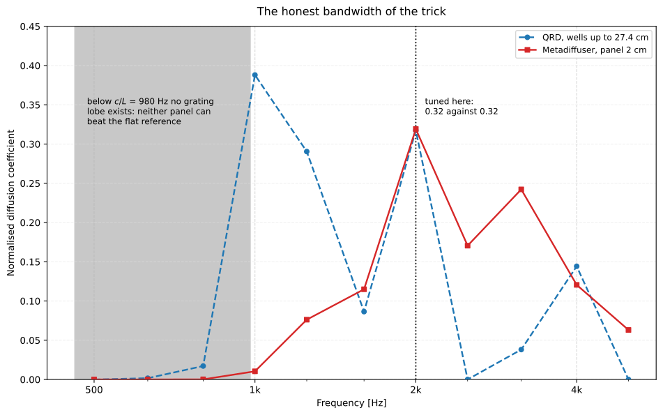
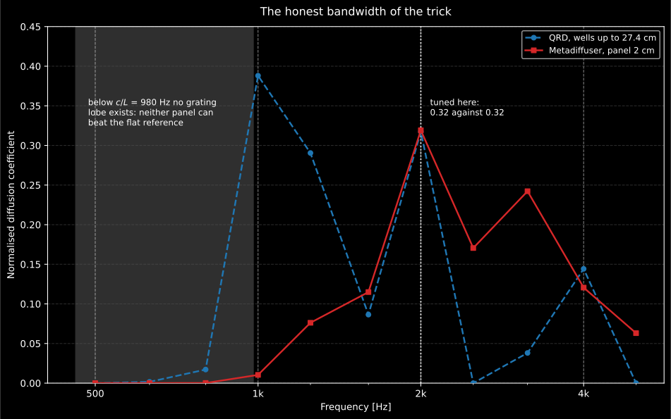
The equivalence is a point, not a band. At 2 kHz the two panels score 0.32 and 0.32; a third of an octave either side they are different surfaces, and the metadiffuser loses the 1 kHz and 1.25 kHz bands the deep grating keeps, because its slits have not yet reached the target phases there. Below Hz the shaded region is not a property of either design: the 35 cm period is shorter than a wavelength, no grating lobe exists to be filled, and the normalised coefficient of any panel of this period collapses towards zero.
Show the code for this figure
import matplotlib.pyplot as plt
# `meta` and `qrd` are the two DiffusionSpectrum objects computed above.fig, ax = plt.subplots()ax.axvspan(bands[0], 343.0 / (5 * 0.07), color="#9e9e9e", alpha=0.16)ax.semilogx(bands, qrd.normalized, "o--", label="QRD, wells up to 27.4 cm")ax.semilogx(bands, meta.normalized, "s-", label="Metadiffuser, panel 2 cm")ax.set_xlabel("Frequency [Hz]")ax.set_ylabel("Normalised diffusion coefficient")ax.legend()plt.show()
The design rule that follows is the one the bullets above imply: tune at the centre of the band the application needs, run this check before committing, and read the single-frequency polar overlay as an illustration rather than a specification.
4. Building one, and checking it
Section titled “4. Building one, and checking it”Everything above is a model of a panel that does not exist yet. Three things stand between the table of millimetres and a surface on a wall.
Fabrication. The chain assumes rigid, smooth, airtight walls. Print or machine in a stiff material and keep the septa between slits thick enough not to flex at the working frequency; a septum that moves adds a compliance the model does not have. Expect printed necks to come out undersized and rougher than drawn, both of which raise the visco-thermal loss inside the resonator and shave , the quantity this design keeps between 0.97 and 1.00, so there is not much of it to give away.
Tolerance. State it in degrees rather than adjectives, using the loop of section 3 backwards: rebuild the panel with one neck side perturbed and read the phase that comes back. On the published slit 1 a mm error on the 6.2 mm neck moves its reflection phase by a few degrees at 2 kHz, which the figure above puts in context: it is small against the dispersion the design already carries across a third of an octave, and large against the 3° the five slits currently sit within.
Verification, at two scales. One cell at a time, metadiffuser_reflection
returns exactly what a two-microphone measurement of that cell in a
rectangular impedance tube one period wide would give, including
well_absorption, so a single slit can be checked before the panel is
committed. That is the
impedance tube method
unchanged. The whole panel is graded on an ISO 17497-2 goniometer, which needs
the six-period 2.1 m array and a flat reference panel of the same footprint
measured under the identical chain; the
diffusers guide gives that
procedure. Because the design is tuned at one frequency, the band-by-band
from that measurement, not the coefficient at 2 kHz, is the
honest grade.
What this guide covers
Section titled “What this guide covers”Covered
The Jiménez et al. (2017) metadiffuser model: the per-well slit and Helmholtz-resonator transfer-matrix chain with visco-thermal effective parameters, end corrections and the slit-radiation term (
metadiffuser_reflection, withMetadiffuserWellandHelmholtzResonatoras the geometry containers andNonewells as flat rigid strips), and its reduction through the Fraunhofer far field to the ISO 17497-2 directional diffusion coefficient (metadiffuser_polar_response) and the band-by-band normalised spectrum (metadiffuser_diffusion_spectrum).Not covered
The model is locally reacting (wells do not couple internally) and shares the stated limits of the Fraunhofer far field: it loses accuracy at low frequency, at grazing angles and where edge diffraction matters, so it grades designs rather than replacing an ISO 17497-2 measurement. The inverse problem (solving resonator geometries for a target phase profile) is not automated; the workflow of section 3 matches phases by evaluation. The critical-coupling design solver for a single slit lives in Metamaterial Absorbers.
References
Section titled “References”- Cox, T. J., & D'Antonio, P. (2017). Acoustic absorbers and diffusers: Theory, design and application (3rd ed.). CRC Press. https://doi.org/10.1201/9781315369211ISBN 978-1-4987-4099-9. The Schroeder sequences, the Fraunhofer far-field model and the diffusion-coefficient machinery the metadiffuser is evaluated with.
- Jiménez, N., Cox, T. J., Groby, J.-P., & Romero-García, V. (2019). Beyond phase grating diffusers using locally-resonant metamaterials. Proceedings of the 23rd International Congress on Acoustics (ICA 2019). The congress companion to the 2017 paper: the transfer-matrix chain, the slow-sound dispersion picture and the far-field comparisons that section 3 condenses.
- Jiménez, N., Cox, T. J., Romero-García, V., & Groby, J.-P. (2017). Metadiffusers: Deep-subwavelength sound diffusers. Scientific Reports, 7, 5389. https://doi.org/10.1038/s41598-017-05710-5The metadiffuser model implemented here: slits loaded by Helmholtz resonators reproduce Schroeder phase profiles and ternary sequences from panels 1/46 to 1/20 of the design wavelength thick, including the quadratic-residue design of section 2.
- Jiménez, N., Groby, J.-P., Pagneux, V., & Romero-García, V. (2017). Iridescent perfect absorption in critically-coupled acoustic metamaterials using the transfer matrix method. Applied Sciences, 7(6), 618. https://doi.org/10.3390/app7060618The slit + Helmholtz-resonator transfer-matrix chain each well is evaluated with, and the critical-coupling condition behind the ternary 0 state.
- Jiménez, N., Huang, W., Romero-García, V., Pagneux, V., & Groby, J.-P. (2016). Ultra-thin metamaterial for perfect and quasi-omnidirectional sound absorption. Applied Physics Letters, 109(12), 121902. https://doi.org/10.1063/1.4962328The resonator impedance (Eq. A23) and its radiation end corrections (Eqs. A24-A27) used in every loaded slit.
- Jiménez, N., Umnova, O., & Groby, J.-P. (Eds.). (2021). Acoustic waves in periodic structures, metamaterials, and porous media. Springer. https://doi.org/10.1007/978-3-030-84300-7Topics in Applied Physics, Vol. 143. The book-length treatment of resonant metamaterial absorbers and diffusers; the modern companion to Cox & D'Antonio for this whole family.