Insulation Ratings (ISO 717)
Standards: ISO 717Key references: Hopkins 2007
Every sound-insulation quantity in this documentation ends its journey the same way: a band spectrum walks in, a single number walks out. Whether the spectrum is a laboratory , a field or , a façade , an impact or , or a flanking , what regulations quote is the weighted single number of ISO 717, and two reference-curve engines produce all of them: ISO 717-1 for airborne quantities, where an unfavourable deviation is a band falling below the reference, and ISO 717-2 for impact quantities, with the sign flipped because a higher impact level is worse. This guide covers the engines themselves: the shifting rule, the spectrum adaptation terms , and , the enlarged-range and one-decimal variants, and the ISO 717 fiche. The measurements that produce the spectra live in the field, laboratory, intensity, survey and flanking guides; the prediction that consumes the ratings is EN 12354.
How do I compute Rw from third-octave sound reduction data in Python?
Section titled “How do I compute Rw from third-octave sound reduction data in Python?”Pass the 16 one-third-octave values from 100 Hz to 3150 Hz to
building.weighted_rating(R). It shifts the ISO 717-1 reference curve and
returns the rating read at 500 Hz, plus the spectrum adaptation terms and
. For the measured spectrum used below, w.rating, w.c, w.ctr prints
30 -2 -3: . The same call rates , and
.
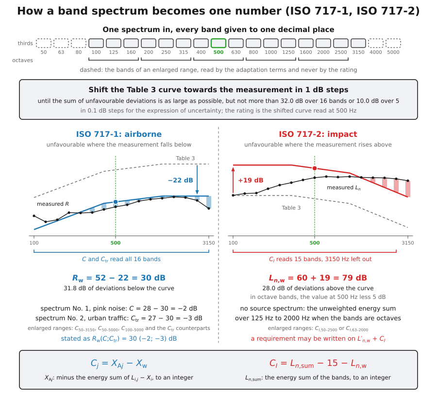
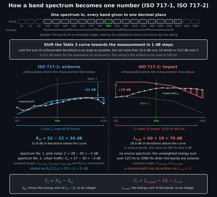
One rule, two engines. Both parts shift their own Table 3 curve the same way, and the shift differs between them only in the side of the curve a deviation counts on: below it for airborne insulation, where the curve comes to rest 22 dB down with 31.8 dB of deviations and reads 30 dB at 500 Hz, and above it for impact sound, where it comes to rest 19 dB up with 28.0 dB and reads 79 dB. Where the bands are octaves, ISO 717-2 takes a further 5 dB off that reading and ISO 717-1 does not. The adaptation terms then go back to the measured bands, all 16 of them for and and only the first 15 for .
Airborne ratings (ISO 717-1)
Section titled “Airborne ratings (ISO 717-1)”The band spectrum is collapsed to one number by the reference-curve method of ISO 717-1: a fixed reference curve is shifted in 1 dB steps toward the measured curve until the sum of unfavourable deviations (where the measurement falls below the reference) is as large as possible but not more than 32.0 dB (16 one-third-octave bands) or 10.0 dB (5 octave bands). The two caps are one rule, not two constants: and , so what the method actually permits is an average unfavourable deviation of 2 dB per band. The rating (, , …) is the shifted reference read at 500 Hz.
The reference curve itself (ISO 717-1:2020, Table 3) is not arbitrary either. It rises 3 dB per one-third octave (9 dB per octave) from 100 Hz to 400 Hz, then 1 dB per one-third octave up to 1250 Hz, and is flat from 1250 Hz up. A rating engine carrying that shape is deliberately lenient at low frequency and unforgiving above 1 kHz, which is why a construction with a low-frequency dip can still rate well, and why exists to put the penalty back. The result object hands you the curve in its shifted position, so the unshifted one is a subtraction away:
import numpy as npfrom phonometry import building
R = [20.4, 16.3, 17.7, 22.6, 22.4, 22.7, 24.8, 26.6,     28.0, 30.5, 31.8, 32.5, 33.4, 33.0, 31.0, 25.5]w = building.weighted_rating(R)
# The curve is shifted until it reads `rating` at 500 Hz; unshifted it reads# 52 dB there, so the shift applied was 52 - rating.reference = np.asarray(w.shifted_reference) + (52 - w.rating)print(w.rating, 52 - w.rating)          # 30 22   (shifted down by 22 dB)print(reference.astype(int).tolist())# [33, 36, 39, 42, 45, 48, 51, 52, 53, 54, 55, 56, 56, 56, 56, 56]
The spectrum adaptation terms (pink noise) and (urban traffic) add the low-frequency penalty of a real source. Both come from one definition (Clause 4.5, Formulae (1) and (2)): re-rate the measured spectrum against a standard source spectrum and subtract the curve-based rating,
where is the level of source spectrum in band (both spectra are A-weighted and normalised to 0 dB overall) and the measured insulation in that band, to one decimal place. The two terms differ only in which spectrum is substituted: No. 1, A-weighted pink noise, representative of living activities (speech, music, radio, television), gives ; No. 2, A-weighted urban road traffic, whose energy sits at low frequency, gives . So the rating plus the term ( for a laboratory index, or for the quantities of the field guide, and likewise with ) is the A-weighted level difference the construction achieves against that source, which is what makes the sum, and not the rating alone, the thing worth specifying. Reading them:
- stays small for most constructions (0 to −2 dB is typical): the pink spectrum is close to the weighting already implicit in the reference curve.
- punishes weak low-frequency insulation. A lightweight double leaf with its mass-air-mass resonance near 100 Hz can carry a of −5 to −10 dB, while a heavy monolithic wall with the same loses far less: two constructions with equal ratings can differ audibly against traffic.
- Design with the descriptor that matches the noise, carried by the field quantity the requirement rates: for a façade on a busy road, (or the plain rating, where the regulation says so) between dwellings, the two example requirements of ISO 717-1, 5.3.
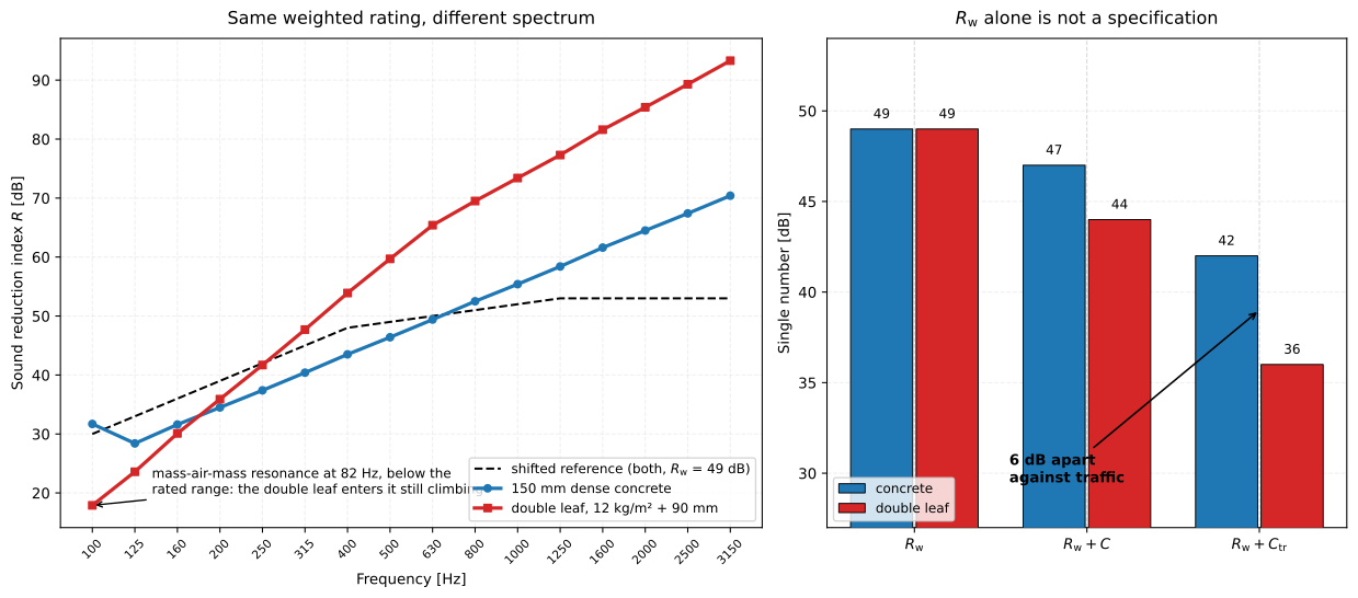
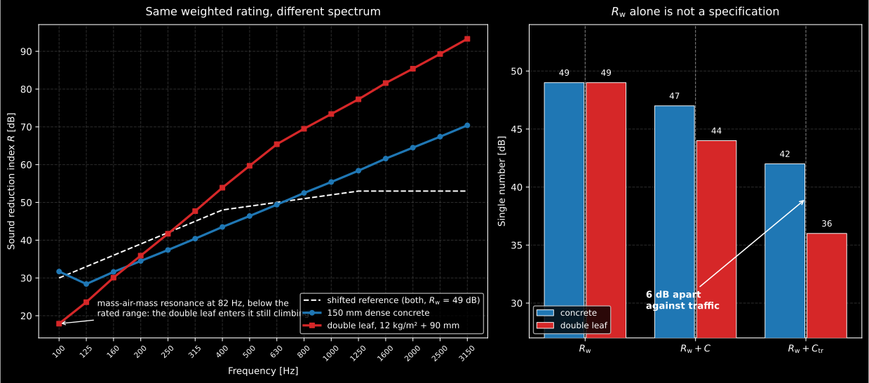
Two constructions, one rating. Both spectra come from the library’s own panel models (Sharp’s method for the concrete leaf, the mass-air-mass double-wall model for the lightweight one), and both rate to dB, so a specification written on alone treats them as interchangeable. They are not: the double leaf enters the rated range still climbing out of its 82 Hz mass-air-mass resonance, and against traffic it gives up 6 dB more than the concrete wall. is what a façade on a busy road is actually specified on.
Show the code for this figure
import matplotlib.pyplot as pltimport numpy as np# `building` is the import of the reference-curve block above.
freqs = np.array([100, 125, 160, 200, 250, 315, 400, 500, 630, 800,                  1000, 1250, 1600, 2000, 2500, 3150], dtype=float)
# 150 mm dense concrete: m' = 2300 x 0.15 = 345 kg/m2, fc = 125 Hz.heavy = np.round(building.single_panel_transmission_loss(    freqs, 345.0, critical_frequency=125.0).transmission_loss, 1)# Metal-stud double leaf: 12 kg/m2 per leaf, 90 mm cavity.light_result = building.double_wall_transmission_loss(freqs, mass1=12.0,                                                      mass2=12.0, gap=0.09)light = np.round(light_result.transmission_loss, 1)
w_heavy = building.weighted_rating(heavy)w_light = building.weighted_rating(light)print(w_heavy.rating, w_heavy.c, w_heavy.ctr)   # 49 -2 -7print(w_light.rating, w_light.c, w_light.ctr)   # 49 -5 -13print(round(light_result.resonance_frequency, 1))            # 81.5 Hz
fig, (ax_spec, ax_bar) = plt.subplots(1, 2, figsize=(13.0, 5.8))x = np.arange(16)ax_spec.plot(x, w_heavy.shifted_reference, "--", label="shifted reference")ax_spec.plot(x, heavy, "-o", label="150 mm dense concrete")ax_spec.plot(x, light, "-s", label="double leaf, 12 kg/m2 + 90 mm")ax_spec.set_xticks(x, [f"{f:g}" for f in freqs], rotation=45, fontsize=8)ax_spec.set(xlabel="Frequency [Hz]", ylabel="Sound reduction index R [dB]")ax_spec.legend()
groups = ("Rw", "Rw + C", "Rw + Ctr")xb = np.arange(3)ax_bar.bar(xb - 0.19, [w_heavy.rating, w_heavy.rating + w_heavy.c,                       w_heavy.rating + w_heavy.ctr], width=0.36,           label="concrete")ax_bar.bar(xb + 0.19, [w_light.rating, w_light.rating + w_light.c,                       w_light.rating + w_light.ctr], width=0.36,           label="double leaf")ax_bar.set_xticks(xb, groups)ax_bar.set_ylabel("Single number [dB]")ax_bar.legend()plt.show()
Every figure of a rating on this page shows the curve where it came to rest. The rule that put it there is iterative, and the two positions that decide the answer are the ones a finished figure has already discarded: the last shift whose unfavourable sum still exceeded 32.0 dB, and the next shift after the answer, which is legal but wastes the allowance. The clip walks both engines through those steps on the two worked spectra of this page.
The reference curve steps in 1 dB increments toward the measured spectrum while the unfavourable deviations shade in band by band and their sum falls toward the 32.0 dB cap. The airborne engine stops at 31.8 dB for Rw = 30 dB, one step before the position that would waste the allowance; the impact engine then runs the same rule with the deviation's sign reversed, the curve stepping upward and stopping at 28.0 dB for Ln,w = 79 dB.
The reference curve steps in 1 dB increments toward the measured spectrum while the unfavourable deviations shade in band by band and their sum falls toward the 32.0 dB cap. The airborne engine stops at 31.8 dB for Rw = 30 dB, one step before the position that would waste the allowance; the impact engine then runs the same rule with the deviation's sign reversed, the curve stepping upward and stopping at 28.0 dB for Ln,w = 79 dB.
Both walks stop where the standard says: at the largest unfavourable sum that does not exceed 32.0 dB. The step before it is rejected for overshooting the cap, and the step after it is legal but reads a decibel lower for no reason, which is what “as large as possible” in ISO 717-1:2020, 4.4 and ISO 717-2:2020, 4.3.1 excludes.
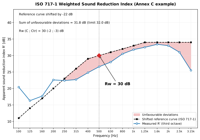
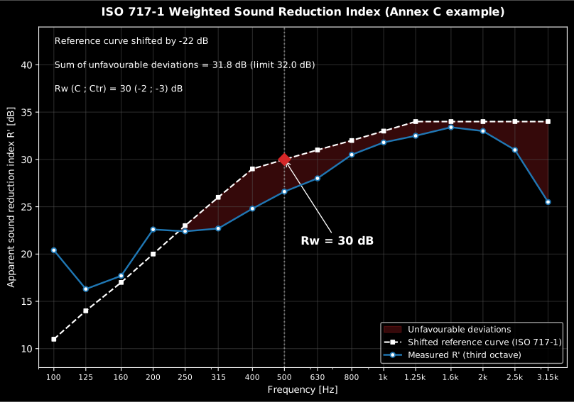
The shifted reference has come to rest where the shaded unfavourable area totals 31.8 dB: one step back would overshoot the cap at 44.1 dB, and one more step down would waste the allowance at 20.6 dB. The rating is then read off that curve at 500 Hz, not off the measurement: the measured spectrum touches 26.6 dB there, and is 30 dB.
# `building`, `R` and `w` come from the reference-curve block above.print(w.rating, w.c, w.ctr)                          # 30 -2 -3  ->  Rw(C;Ctr) = 30(-2;-3)print(w.unfavourable_sum)                            # 31.8  (cap 32.0 = 2.0 x 16)
w.plot()   # measured R vs shifted ISO 717-1 reference, deviations shaded (needs matplotlib)
Show the code for this figure
import matplotlib.pyplot as pltfrom phonometry import building
# Single-number rating from a measured 16-band R spectrum (ISO 717-1 Annex C)R = [20.4, 16.3, 17.7, 22.6, 22.4, 22.7, 24.8, 26.6,     28.0, 30.5, 31.8, 32.5, 33.4, 33.0, 31.0, 25.5]w = building.weighted_rating(R)
# One line — measured curve vs the shifted ISO 717-1 reference, deviations shaded:w.plot()plt.show()
# By hand, from the band curve the result now carries:fig, ax = plt.subplots()ax.semilogx(w.band_centers, w.measured, "o-", label="Measured R")ax.semilogx(w.band_centers, w.shifted_reference, "s--", label="Shifted reference")ax.fill_between(w.band_centers, w.measured, w.shifted_reference,                where=w.measured < w.shifted_reference, interpolate=True,                alpha=0.3, label="Unfavourable deviations")ax.set_xlabel("Frequency [Hz]")ax.set_ylabel("Sound reduction index [dB]")ax.set_title(f"Rw = {w.rating} dB  (C={w.c:+d}; Ctr={w.ctr:+d})")ax.legend()plt.show()
weighted_rating() parameters
Section titled “weighted_rating() parameters”| Parameter | Type | Units | Range / default | Notes |
|---|---|---|---|---|
values_by_band | 1D array | dB | 16 (thirds) or 5 (octaves) | Measured , , … per band |
bands | str or None | — | 'third-octave' / 'octave' / None | None infers from the count |
weighted_rating() returns a WeightedRatingResult (rating, c, ctr,
unfavourable_sum, all integers except the sum), plus the three fields the
figures on this page are drawn from: band_centers, measured and
shifted_reference, and quantity naming what was rated.
Impact ratings (ISO 717-2)
Section titled “Impact ratings (ISO 717-2)”The single-number rating (ISO 717-2) shifts the same style of reference curve, but an unfavourable deviation now occurs where the measurement exceeds the reference (impact noise is worse when higher), the sign opposite to ISO 717-1. The rating (, , ) is the shifted reference read at 500 Hz; for octave bands it is then reduced by 5 dB. The spectrum adaptation term (ISO 717-2:2020 Formulae (A.1) to (A.3)) uses the energetic sum over 100–2500 Hz (the first 15 thirds, excluding 3150 Hz) or 125–2000 Hz (octaves).
The dB is a normalising offset, not physics: it is chosen so that comes out about zero for a massive floor with an effective covering, slightly positive for a timber joist floor whose low-frequency peaks dominate, and down to dB for a bare or poorly covered concrete floor (Annex A.1). Read that way, the dB of the example below says the measured spectrum is far flatter and more high-frequency-weighted than the reference contour (a bare slab, not a floor with a covering), so the floor is better at the low frequencies footsteps excite than dB alone suggests. The corollary is a design trap: a soft covering acts where the reference curve is most demanding, so it improves the single number more than it improves what the neighbour hears. The unweighted sum is built on exists precisely because it correlates better with A-weighted walking noise than the reference-curve rating does, which is why requirements are sometimes written on rather than on .
For measurements extended down to 50 Hz,
weighted_impact_rating_extended additionally returns the enlarged-range
term (A.2.1 NOTE), and with one_decimal=True the
0.1 dB-step rating used in uncertainty statements (it reproduces the printed
dB and dB of A.2.2).
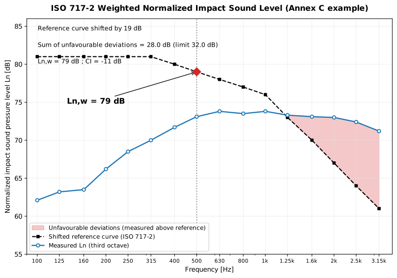
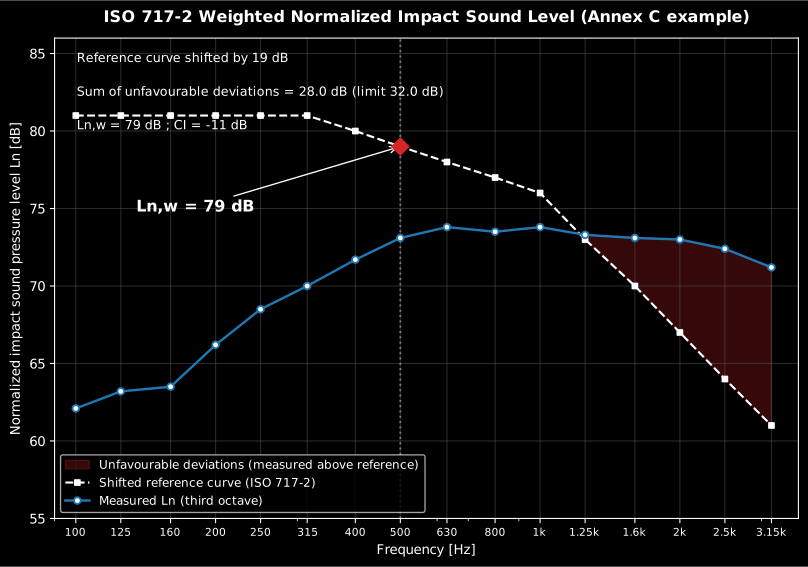
The same fitting rule with the sign reversed: the shaded area is where the measurement rises above the reference, and the curve is shifted up until that area reaches 28.0 dB against the same 32.0 dB cap. A floor rated this way is worse the higher its number.
import numpy as npfrom phonometry import building
# ISO 717-2 Annex C worked example: the bare heavy floor of Table C.1,# laboratory Ln in one-third octaves. CI is read over the 100-2500 Hz sum# that A.2.1 asks for, not over the sixteen bands the 2020 print of that# cell sums.l_n = np.array([62.1, 63.2, 63.5, 66.2, 68.5, 70.0, 71.7, 73.1,                73.8, 73.5, 73.8, 73.3, 73.1, 73.0, 72.4, 71.2])
# Weighted impact rating + spectrum adaptation term CI (ISO 717-2)res_imp = building.weighted_impact_rating(l_n)print(res_imp.rating, res_imp.ci, res_imp.unfavourable_sum)   # 79 -11 28.0  ->  Ln,w(CI)=79(-11)
# Octave-band data carry the extra -5 dB reduction (Clause 4.3.2)octave = np.array([65.3, 64.5, 58.0, 55.8, 43.0])print(building.weighted_impact_rating(octave).rating)  # 54
res_imp.plot()   # measured Ln vs shifted ISO 717-2 reference, measured-above shaded (needs matplotlib)
Show the code for this figure
import matplotlib.pyplot as pltimport numpy as npfrom phonometry import building
# 16 one-third-octave impact levels Ln, dB (ISO 717-2 Annex C worked# example, the bare heavy floor of Table C.1; the CI in the title is read# over the 100-2500 Hz sum that A.2.1 asks for).l_n = np.array([62.1, 63.2, 63.5, 66.2, 68.5, 70.0, 71.7, 73.1,                73.8, 73.5, 73.8, 73.3, 73.1, 73.0, 72.4, 71.2])# Weighted impact rating + spectrum adaptation term CI (ISO 717-2)res_imp = building.weighted_impact_rating(l_n)
# One line — measured Ln vs the shifted ISO 717-2 reference (measured-above shaded):res_imp.plot()plt.show()
# By hand, from the band curve the result now carries (note the opposite sign:# an unfavourable deviation is where the MEASURED level exceeds the reference).# Here the input was Ln, so the rated quantity is Ln,w:fig, ax = plt.subplots()ax.semilogx(res_imp.band_centers, res_imp.measured, "o-", label="Measured Ln")ax.semilogx(res_imp.band_centers, res_imp.shifted_reference, "s--", label="Shifted reference")ax.fill_between(res_imp.band_centers, res_imp.shifted_reference, res_imp.measured,                where=res_imp.measured > res_imp.shifted_reference, interpolate=True,                alpha=0.3, label="Unfavourable deviations")ax.set_xlabel("Frequency [Hz]")ax.set_ylabel("Impact sound pressure level [dB]")ax.set_title(f"Ln,w = {res_imp.rating} dB  (CI={res_imp.ci:+d})")ax.legend()plt.show()
Feeding this spectrum into weighted_impact_rating reproduces the ISO 717-2
Annex C rating (thirds ; octave 54, )
and, reading over the 100–2500 Hz sum that A.2.1 specifies,
for the thirds. The 2020 print of Table C.1 sums all
sixteen bands in that cell and gives instead; the registry entry is in
Errata.
weighted_impact_rating() parameters
Section titled “weighted_impact_rating() parameters”| Parameter | Type | Units | Range / default | Notes |
|---|---|---|---|---|
values_by_band | 1D array | dB | 16 (thirds) or 5 (octaves) | Measured , or per band |
bands | str or None | — | 'third-octave' / 'octave' / None | None infers from the count |
weighted_impact_rating() returns an ImpactRatingResult (rating,
ci integers, unfavourable_sum in dB), with the same three plotting fields
as the airborne result: band_centers, measured and shifted_reference.
Enlarged frequency ranges and one-decimal ratings
Section titled “Enlarged frequency ranges and one-decimal ratings”When the measurement covers more than the core 100–3150 Hz bands, ISO 717-1
Annex B defines additional adaptation terms with the range as a subscript
(, , and the
counterparts), computed with the Table B.1 spectra over the enlarged
range. weighted_rating_extended takes the band values with their centre
frequencies and returns the core rating plus every extended term the input
covers (the impact counterpart weighted_impact_rating_extended adds
). With one_decimal=True the reference curve shifts in
0.1 dB steps and all reductions keep one decimal: the variant ISO 717
prescribes “for the expression of uncertainty” and ISO 12999-1 Annex B
requires when stating the uncertainty of a single-number value.
Where those extra bands come from matters as much as what the term does with them. In a room whose volume, to the nearest cubic metre, is under 25 m³, ISO 16283 does not let the 50 Hz, 63 Hz and 80 Hz bands be measured with the default procedure alone: the corner procedure is mandatory there, and it can move those three bands by several decibels, which can move by a whole one. So a requirement written as is judged on the corner procedure whether the report mentions it or not. See Small Rooms: the ISO 16283 Low-Frequency Procedure.
from phonometry import building
# Single-number rating from a measured 16-band R spectrum (ISO 717-1 Annex C)R = [20.4, 16.3, 17.7, 22.6, 22.4, 22.7, 24.8, 26.6,     28.0, 30.5, 31.8, 32.5, 33.4, 33.0, 31.0, 25.5]
freqs = [50, 63, 80, 100, 125, 160, 200, 250, 315, 400, 500,         630, 800, 1000, 1250, 1600, 2000, 2500, 3150, 4000, 5000]r_ext = [18.7, 19.2, 20.0, *R, 26.8, 29.2]     # ISO 717-1 Annex C, Table C.2ext = building.weighted_rating_extended(r_ext, freqs)print(ext.rating, ext.c, ext.ctr, ext.c_50_5000, ext.ctr_50_5000)# 30 -2 -3 -2 -4   ->  Rw(C;Ctr;C50-5000;Ctr,50-5000) = 30(-2;-3;-2;-4)
one_dp = building.weighted_rating_extended(r_ext, freqs, one_decimal=True)print(one_dp.rating)   # 30.0, the 0.1 dB-step rating for uncertainty statements
ext.plot()   # enlarged-range curve vs the shifted core reference, Annex B terms in the title (needs matplotlib)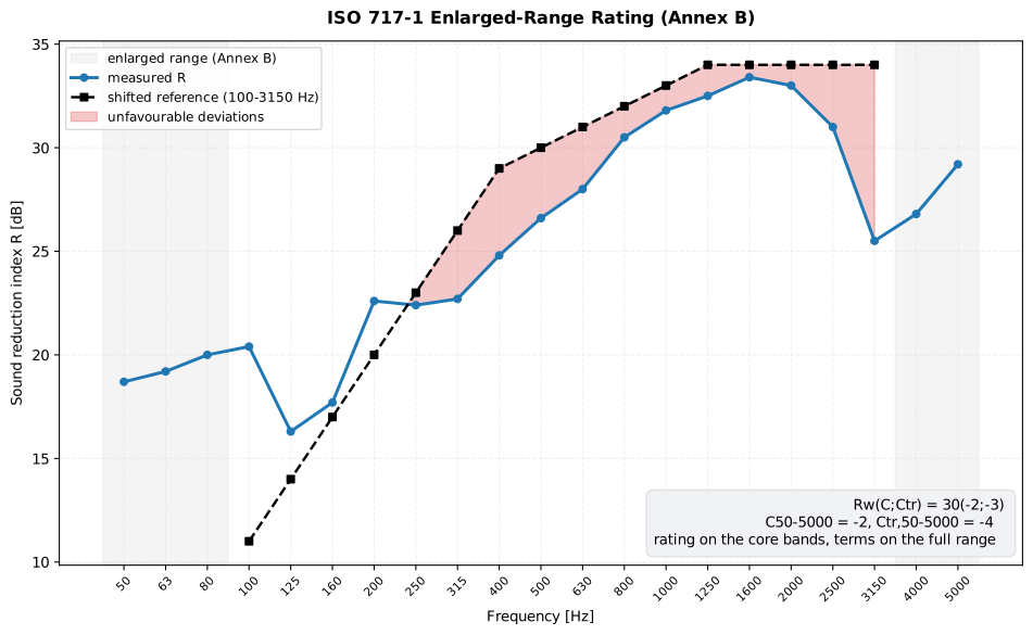
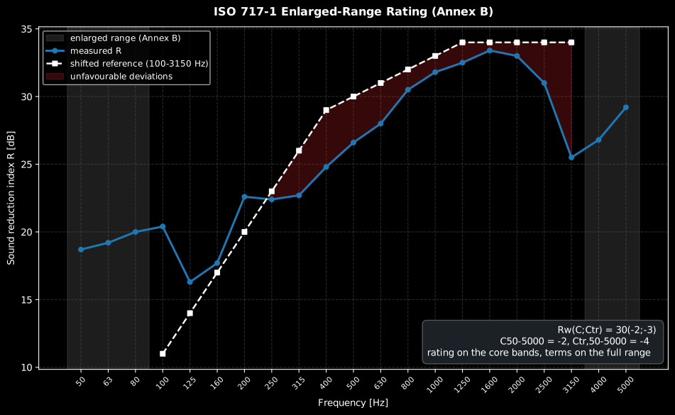
The rating itself is still evaluated on the 16 core bands (100–3150 Hz); the enlarged bands only enter the Annex B adaptation terms, so the shifted reference curve stops at the core-range edges while the measured curve continues into the shaded enlarged range.
Show the code for this figure
import matplotlib.pyplot as pltfrom phonometry import building
# Single-number rating from a measured 16-band R spectrum (ISO 717-1 Annex C)R = [20.4, 16.3, 17.7, 22.6, 22.4, 22.7, 24.8, 26.6,     28.0, 30.5, 31.8, 32.5, 33.4, 33.0, 31.0, 25.5]freqs = [50, 63, 80, 100, 125, 160, 200, 250, 315, 400, 500,         630, 800, 1000, 1250, 1600, 2000, 2500, 3150, 4000, 5000]r_ext = [18.7, 19.2, 20.0, *R, 26.8, 29.2]     # ISO 717-1 Annex C, Table C.2ext = building.weighted_rating_extended(r_ext, freqs)
# One line — the enlarged-range curve vs the shifted core reference:ext.plot()plt.show()
# By hand, from the band curves the result carries (the full enlarged-range# curve on ext, the core-band reference on ext.core):fig, ax = plt.subplots()ax.semilogx(ext.band_centers, ext.measured, "o-", label="Measured R")ax.semilogx(ext.core.band_centers, ext.core.shifted_reference, "s--",            label="Shifted reference (core bands)")ax.fill_between(ext.core.band_centers, ext.core.measured,                ext.core.shifted_reference,                where=ext.core.measured < ext.core.shifted_reference,                interpolate=True, alpha=0.3, label="Unfavourable deviations")ax.set_xlabel("Frequency [Hz]")ax.set_ylabel("Sound reduction index [dB]")ax.set_title(f"Rw = {ext.rating} dB  (C50-5000={ext.c_50_5000:+g}; "             f"Ctr,50-5000={ext.ctr_50_5000:+g})")ax.legend()plt.show()
ISO 717 report (.report())
Section titled “ISO 717 report (.report())”Both rating results render a one-page PDF fiche laid out like an
accredited-laboratory test report through a report(path) method: a
standard-basis line (measurement standard plus the ISO 717 rating part), an
optional metadata header block, the one-third-octave table beside the
measured-versus-shifted-reference plot (the result’s own .plot()), the boxed
single-number result, an optional verdict row and a footer with the fixed
disclaimer. WeightedRatingResult.report() labels the airborne ISO 717-1 fiche
(, deviations where the reference is above the measurement);
ImpactRatingResult.report() labels the impact ISO 717-2 fiche
(, deviations the opposite way).
SoundReductionResult.report() is a convenience that rates the predicted
and writes its fiche in one call; that result comes from the EN 12354
panel models of
Panel sound insulation,
so it is the one entry point here whose input was never measured.
The report metadata is supplied as a ReportMetadata frozen dataclass (every
field optional; only the supplied fields are rendered, and the numeric fields
must satisfy their field-specific physical ranges, detailed in the table
below). Passing metadata=None produces a lightweight
prediction fiche (body, result and disclaimer only). When
metadata.requirement is set, a verdict row is added: an airborne rating passes
when it is at or above the requirement, an impact rating when it is at or below
it (a lower impact level is better). Setting verbose=True swaps the two-column
f | value table for the ISO 717 Annex C columns (frequency, measured value,
shifted reference, unfavourable deviation).
Rendering needs reportlab, kept out of the runtime dependencies as the optional
phonometry[report] extra (pip install phonometry[report]); a missing
reportlab raises a clear ImportError with the install command, and the plot
still needs matplotlib (phonometry[plot]). Only engine="reportlab" is
supported; any other engine raises ValueError. The fiche renders in English by
default; pass language="es" for a Spanish fiche (translated fixed strings and
a comma decimal separator), e.g.
building.weighted_rating(R).report("Rw_fiche_es.pdf", language="es").
from phonometry import building, ReportMetadata
# Airborne rating from a measured 16-band R spectrum (ISO 717-1)R = [20.4, 16.3, 17.7, 22.6, 22.4, 22.7, 24.8, 26.6,     28.0, 30.5, 31.8, 32.5, 33.4, 33.0, 31.0, 25.5]metadata = ReportMetadata(    specimen="200 mm reinforced-concrete wall",    client="Acoustic Test Client Ltd.",    area=10.0, mass_per_area=460.0,    source_volume=53.0, receiving_volume=51.0,    temperature_c=21.5, relative_humidity_percent=45.0, static_pressure_kpa=101.3,    test_room="Transmission suite T1",    measurement_standard="ISO 10140-2",    test_date="2026-07-18",    laboratory="Phonometry Reference Laboratory",    operator="José Manuel Requena Plens",    report_id="PHN-2026-0042",    requirement=42.0,          # adds the PASS/FAIL verdict row)building.weighted_rating(R).report(    "Rw_fiche.pdf", metadata=metadata)                                                           # Rw (C; Ctr)
# Impact rating from a measured 16-band L'nT spectrum (ISO 717-2)l_nt = [45.0, 47.0, 48.0, 49.0, 51.0, 52.0, 53.0, 54.0,        55.0, 56.0, 57.0, 58.0, 55.0, 52.0, 49.0, 46.0]building.weighted_impact_rating(l_nt).report("Lnw_fiche.pdf")  # Ln,w (CI)
Both example fiches are regenerated with make reports and kept rendered in the
repository; click either preview to open the PDF.
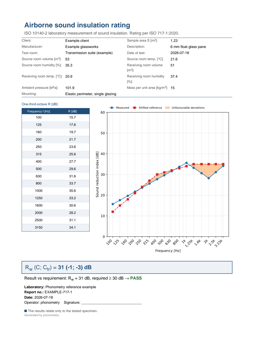
One-page airborne sound insulation fiche: a metadata header (client, specimen, sample area, room volumes, per-room temperature and humidity, ambient pressure and mounting), the one-third-octave R table beside the measured-versus-shifted-reference plot, the boxed Rw (C; Ctr) single-number result and a PASS verdict against the 30 dB requirement.
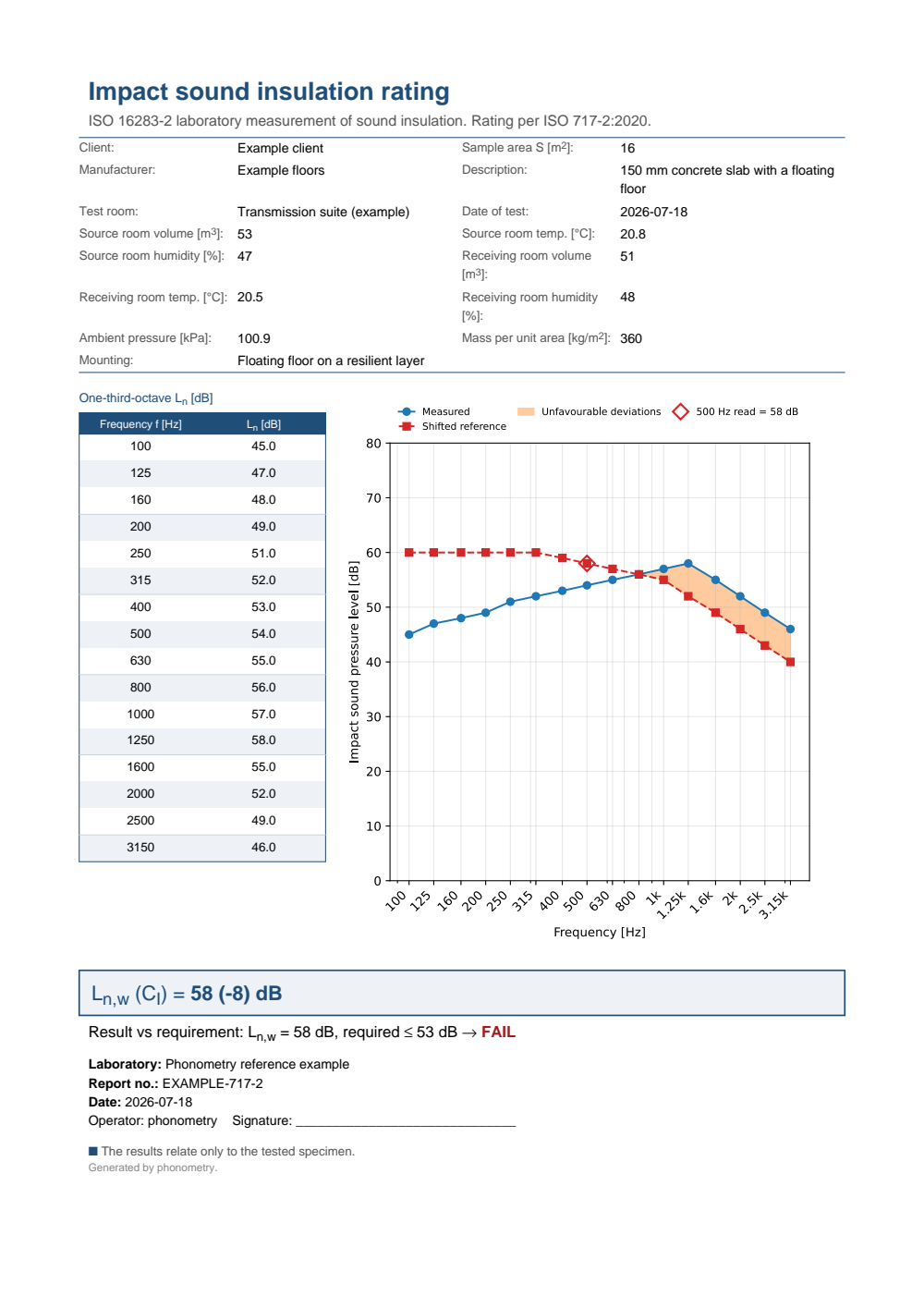
One-page impact sound insulation fiche in the same accredited layout for the normalized impact sound pressure level Ln: the metadata header, the one-third-octave Ln table beside the measured-versus-shifted-reference plot with the 500 Hz read-off, the boxed Ln,w (CI) single-number result and a FAIL verdict against the 53 dB requirement (a lower impact level is better).
Report metadata (ReportMetadata)
Section titled “Report metadata (ReportMetadata)”Every field is optional and only the supplied ones are rendered, so the same object drives a full accredited fiche and a lightweight prediction fiche. The numeric fields are validated on construction by physical range.
| Field | Type | Rendered as |
|---|---|---|
specimen, client, mounted_by, manufacturer | str | Header identity of the tested element and who it was tested for / mounted by |
area, mass_per_area | float > 0 | Sample area (m²) and measured mass per unit area (kg/m²) |
source_volume, receiving_volume | float > 0 | Room volumes (m³) |
temperature_c, relative_humidity_percent | float | Single representative climate: air temperature (°C, any sign), relative humidity (0–100 %) |
static_pressure_kpa | float > 0 | Ambient (static) air pressure during the test (kPa) |
source_temperature_c, source_relative_humidity_percent, receiving_temperature_c, receiving_relative_humidity_percent | float | Per-room climate when source and receiving rooms are reported separately (same ranges as above) |
test_room, mounting, measurement_standard, test_date | str | Facility, mounting condition, the measurement standard (forms the standard-basis line) and the test date |
laboratory, operator, report_id, notes | str | Footer: institute, operator signature line, report number and free-form remarks |
requirement | float | Target single number; adds the verdict row (airborne passes at or above it, impact at or below it) |
What this guide covers
Section titled “What this guide covers”Covered
ISO 717-1:2020’s reference-curve airborne rating (the 1 dB shifting rule with the 32.0 dB / 10.0 dB unfavourable-deviation caps, read at 500 Hz) with the Annex A spectrum adaptation terms and , via
building.weighted_rating; ISO 717-2:2020’s impact rating with the opposite deviation sign, the octave −5 dB reduction and the term, viabuilding.weighted_impact_rating; the Annex B / A.2.1 enlarged-range terms and the 0.1 dB-step one-decimal variants viabuilding.weighted_rating_extendedandbuilding.weighted_impact_rating_extended; and the ISO 717 fiche through.report()with the sharedReportMetadatacontainer. Conformance is anchored on the standards’ own Annex C worked examples.Not covered
Nothing on this page measures: every function takes an already-measured (or predicted) band spectrum from the field, laboratory, intensity, survey or flanking guides. The façade single number of ISO 16283-3 Annex F and the flanking reuse these engines from their own guides rather than duplicating them. One member of the ISO 717 family is deliberately absent: the A-weighted maximum impact level of ISO 717-2:2020 Annex D, which rates the rubber ball and the bang machine. It shifts no curve at all (it is an energy sum of A-weighted band levels), so it is not produced by either engine on this page and lives with the sources it rates, in Heavy and Soft Impact Sources.
Quick answers
Section titled “Quick answers”What is the difference between the C and Ctr spectrum adaptation terms?
Section titled “What is the difference between the C and Ctr spectrum adaptation terms?”Both re-rate the same measured curve against the two source spectra of ISO 717-1 Annex A: against A-weighted pink noise (living activities: speech, music, radio, television) and against A-weighted urban road traffic, whose energy sits at low frequency. is typically 0 to −2 dB, while a lightweight double leaf with a mass-air-mass resonance near 100 Hz can carry a of −5 to −10 dB.
References
Section titled “References”- Hopkins, C. (2007). Sound insulation. Butterworth-Heinemann. https://doi.org/10.4324/9780080550473The interpretation of the single-number ratings and what they hide about the underlying band spectra. ISBN 978-0-7506-6526-1.
- International Organization for Standardization. (2020). Acoustics — Rating of sound insulation in buildings and of building elements — Part 1: Airborne sound insulation (ISO 717-1:2020). The reference-curve rating and the spectrum adaptation terms C and Ctr interpreted above; also the single-number engine for the façade quantity (Annex F).
- International Organization for Standardization. (2020). Acoustics — Rating of sound insulation in buildings and of building elements — Part 2: Impact sound insulation (ISO 717-2:2020). The impact reference-curve rating and the spectrum adaptation term CI, with the enlarged-range CI,50-2500 term.