Sound Insulation by Intensity (ISO 15186)
Standards: ISO 15186Key references: Hopkins 2007
A reverberation room reads transmitted sound power indirectly: the receiving room integrates every watt that arrives, whichever path carried it, and the absorption area converts the room level back into a power. The sound-intensity method of ISO 15186 replaces that inference with a direct reading: a p-p intensity probe scans a measurement surface that encloses the specimen and measures the power radiated by the test element alone, so flanking transmission stays out of the number. This guide covers the intensity sound reduction index and its -modified form, the element-normalized level difference of small building elements, the surface qualification indicator and the accredited test fiches. The pressure-based laboratory chain lives in Laboratory Insulation Measurement; the probe physics and its field indicators are the subject of the Sound Intensity guide.
Measuring the transmitted power directly (ISO 15186-1)
Section titled “Measuring the transmitted power directly (ISO 15186-1)”The quantity being measured is a surface integral: the net sound power crossing an imaginary surface drawn around the radiating face of the specimen, , where is the time-averaged intensity vector and the outward normal. Two consequences follow, and between them they are the whole method. First, a source outside the closed surface contributes nothing to the integral: what enters through one face leaves through another, so a flanking wall radiating into the same receiving room cancels itself out and only the enclosed specimen survives. Second, the sign matters: a patch of surface where energy is flowing back towards the specimen subtracts, which is why the standard carries a minus-sign rule (Clause 6.4.6) that no pressure-based method needs. The probe reads point by point and the operator performs the integration by moving it, which makes the scan pattern part of the measurement rather than a matter of technique.
That is what the pressure method cannot do. It reads the transmitted power indirectly, from the receiving-room level and its absorption area, and the room integrates every watt that arrives whichever path carried it. The intensity method is therefore the tool of choice when flanking is high (ISO 15186-1:2000, Clause 1). From the source-room level and the average normal intensity level over the surface (area ), for a specimen of area ,
where the dB is the diffuse-field offset between the sound pressure level and the incident intensity level. The same formula gives the apparent index in the field (ISO 15186-2). The intensity scan measures the transmitted power directly. The reverberation-room pressure method does not: it infers the power from the receiving-room level and so underestimates it, which makes the ISO 10140-2 come out slightly high. The modified index adds that same bias back to the intensity result, so an intensity measurement can be quoted against pressure-method data (ISO 15186-1, Clause 3.10 NOTE 1). Report when the aim is the true transmitted power; report when the aim is comparability with an ISO 10140-2 result. Earlier revisions of this guide blamed the bias on the intensity method itself, which would have called for subtracting , not adding it. The adaptation term (Annex B) is for a well-defined room, or the room-independent . The first form is the Waterhouse boundary-energy term, which makes the second readable as that same term evaluated at a fixed . For small elements the element normalized level difference replaces with (, element units).
import numpy as npfrom phonometry import building
# Source-room level Lp1 and the average normal intensity level LIn over the# measurement surface (Sm), for a specimen of area S; 16 one-third-octave bands.lp1 = np.full(16, 85.0)l_in = np.full(16, 40.0)freqs = [100, 125, 160, 200, 250, 315, 400, 500, 630, 800,         1000, 1250, 1600, 2000, 2500, 3150]   # nominal 1/3-octave centreskc = building.adaptation_term_kc(freqs)                  # Annex B (B.2)res = building.intensity_sound_reduction(lp1, l_in, measurement_area=12.0, area=10.0, kc=kc)print(round(float(res.r_i[0]), 2))          # 38.21  RI = Lp1 - 6 - [LIn + 10 lg(Sm/S)]print(round(float(res.r_i_modified[0]), 2)) # 40.29  RI,M = RI + Kcprint(res.rating.rating)                     # 38  ->  RI,w (ISO 717-1 engine)
# Qualify the measurement surface: FpI = Lp - LIn must stay < 10 dB (< 6 dB when# the receiving side is absorbing); the probe's residual index must exceed FpI+10.# Lp is the receiving-room pressure level measured over the same surface, if# possible simultaneously with the scan (Clause 6.4.2). Here it sits 6 dB above# LIn, i.e. exactly on the absorbing-specimen criterion.fpi = building.surface_pressure_intensity_indicator(np.full(16, 46.0), l_in)print(round(float(fpi[0]), 1))               # 6.0
res.plot()   # measured RI vs shifted ISO 717-1 reference (needs matplotlib)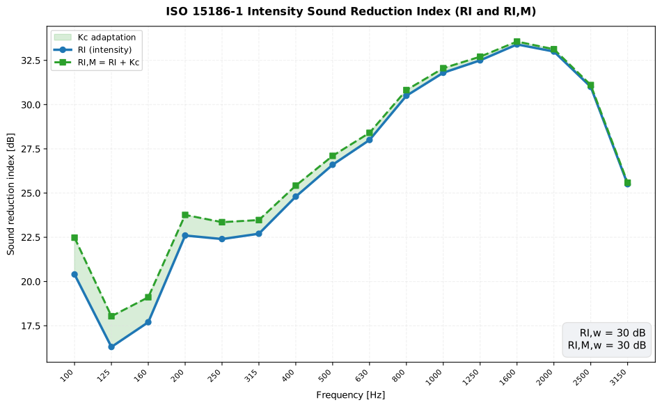
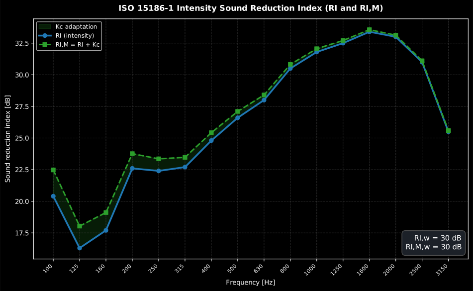
The modified index lifts (most at the low bands, where is largest), so an intensity measurement reproduces the ISO 10140-2 pressure result. The automatic rating is formed only for exactly 16 one-third-octave or 5 octave values.
Show the code for this figure
import matplotlib.pyplot as pltimport numpy as npfrom phonometry import building
# A light wall: source-room SPL Lp1 = 85 dB and the measured normal intensity# level LIn over the Sm = 12 m2 surface, 16 one-third-octave bands.freqs = [100, 125, 160, 200, 250, 315, 400, 500, 630, 800,         1000, 1250, 1600, 2000, 2500, 3150]l_in = np.array([57.8, 61.9, 60.5, 55.6, 55.8, 55.5, 53.4, 51.6,                 50.2, 47.7, 46.4, 45.7, 44.8, 45.2, 47.2, 52.7])kc = building.adaptation_term_kc(freqs)           # Annex B adaptation termres = building.intensity_sound_reduction(np.full(16, 85.0), l_in,                                         measurement_area=12.0, area=10.0,                                         kc=kc)
x = np.arange(len(freqs))fig, ax = plt.subplots()ax.fill_between(x, res.r_i, res.r_i_modified, alpha=0.2, label="Kc adaptation")ax.plot(x, res.r_i, "-o", label="RI (intensity)")ax.plot(x, res.r_i_modified, "--s", label="RI,M = RI + Kc")ax.set_xticks(x, [str(f) for f in freqs], rotation=45)ax.set(xlabel="Frequency [Hz]", ylabel="Sound reduction index [dB]",       title=f"RI,w = {res.rating.rating} dB, RI,M,w = {res.rating_modified.rating} dB")ax.legend()plt.show()
Scanning the measurement surface (Clause 6.4)
Section titled “Scanning the measurement surface (Clause 6.4)”A method defined by how a probe is moved is not documented by its formula. Everything below fixes a number that the formula then consumes, and none of it is checked by the functions on this page.
How the measurement goes
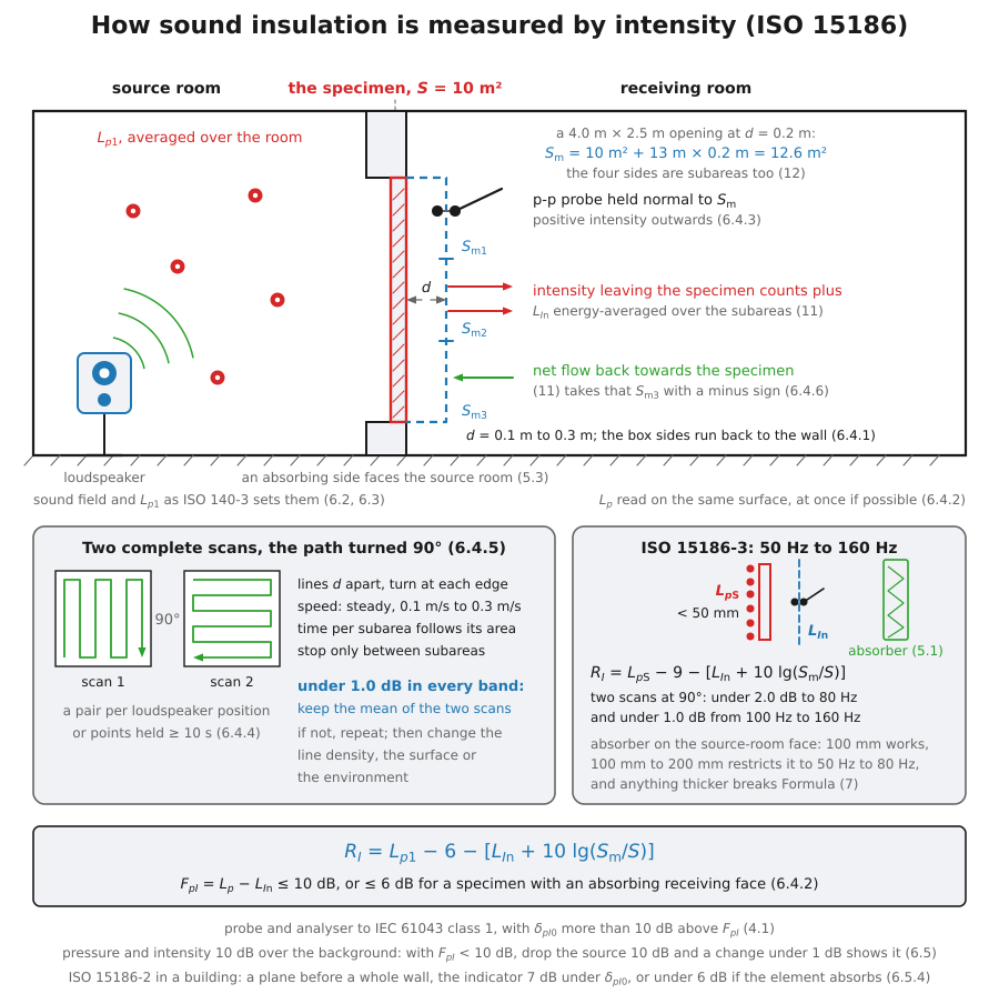
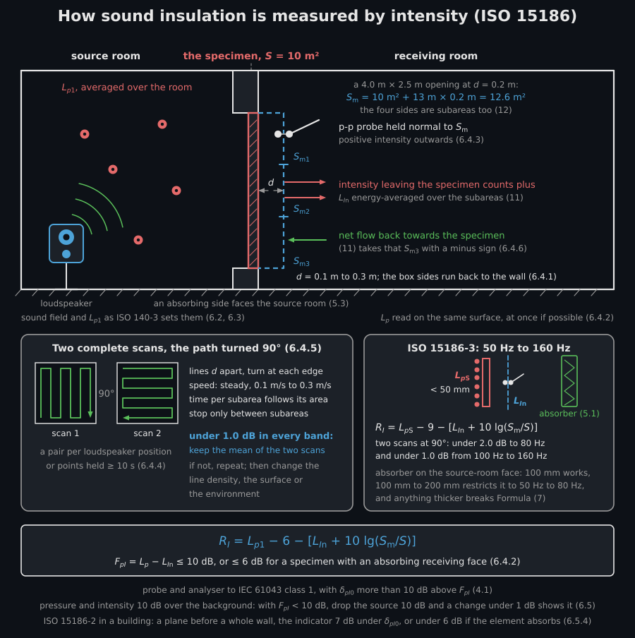
Section titled “How the measurement goes”The analyser and its probe have to meet IEC 61043 class 1, with a pressure-residual intensity index more than 10 dB above the you expect. Before each use, let the instrument warm up, set both microphones with a class 0 or class 1 sound calibrator, and measure the residual index on the residual-intensity testing device. Drive the source room and take as ISO 140-3 asks. On the receiving side, the measurement surface is the flat opening of a niche at least 0.1 m deep, and otherwise a box, at a measurement distance of 0.1 m to 0.3 m. Scan it with the probe normal to the surface and reading outwards, in lines about one measurement distance apart, at a constant 0.1 m/s to 0.3 m/s, giving each subarea time in proportion to its area. A negative intensity, or above 10 dB (6 dB for a specimen whose receiving face absorbs), means moving the surface out by 5 cm to 10 cm before adding absorption. Scan again with the path turned 90°: the mean of the pair stands only if the two differ by less than 1.0 dB in every band. With below 10 dB, lower the source by 10 dB: if moves by less than 1 dB, both levels clear the background by 10 dB. Report to one decimal beside and the residual index in every band, with , , the measurement distance and the probe’s microphones and spacer.
The surface (Clause 6.4.1). The measurement surface totally encloses the test specimen. A specimen in a niche deeper than 0.1 m is normally measured on the flat surface of the niche opening; otherwise, and for most small building elements, the surface is box-shaped. Choose the measurement distance in the 0.1 m to 0.3 m band. Below 0.1 m the near field of the vibrating element makes the intensity change sign repeatedly, so the integral stops converging; above 0.3 m a box-shaped surface picks up too much of the room.
Qualifying the surface (Clause 6.4.2). Measure and, if possible simultaneously, the surface-averaged pressure level , and form the surface pressure-intensity indicator (Formula (10)). The surface fails qualification if the measured intensity is negative, or if dB for a sound-reflecting specimen or dB for one with an absorbing surface facing the receiving room. The remedy is ordered: first increase the measurement distance by 5 cm to 10 cm; only if that fails, add absorption to the receiving room. The criterion applies per scan and per loudspeaker position, and to the total surface, not to individual subareas (for discrete positions, to the surface average). The standard’s rule of thumb for how much absorption is enough is , with the measurement surface and the receiving room’s absorption area, and the more flanking there is the larger has to be.
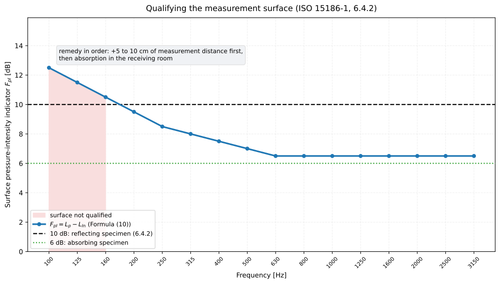
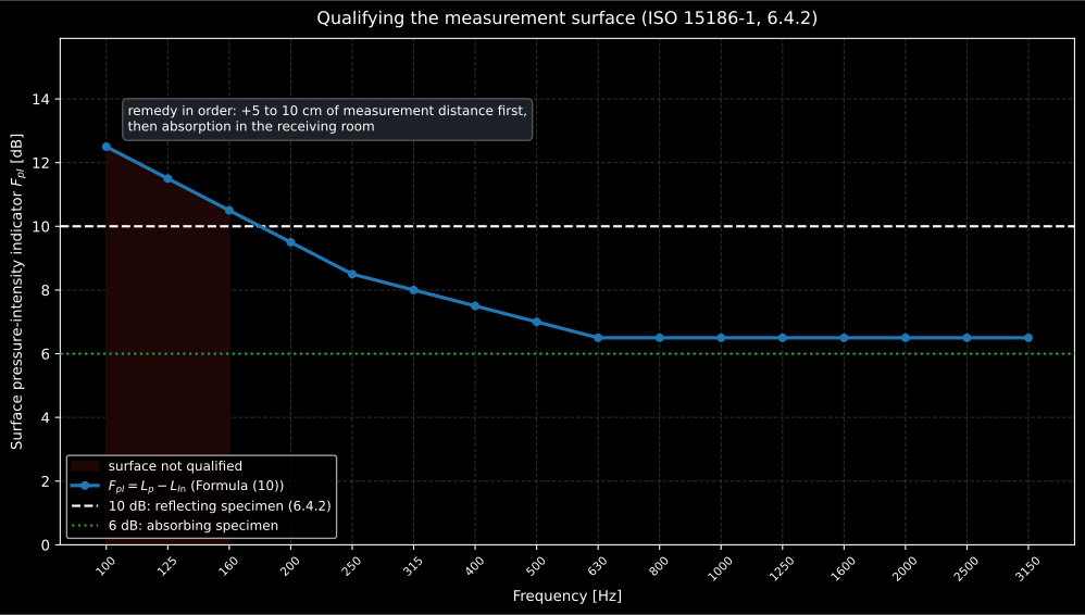
Qualification is per band, and it fails where a receiving room is least absorbent. Here the three lowest bands sit above the 10 dB line, so the surface is not qualified for a reflecting specimen at all and the scan is not yet a result; and even the qualified part sits above the 6 dB line, so this surface could not be used for a specimen with an absorbing face. The remedy is ordered by the standard: add 5 cm to 10 cm of measurement distance first, and only then put absorption into the receiving room.
Show the code for this figure
import matplotlib.pyplot as plt# `np` and `building` are the imports of the first block above.
freqs = [100, 125, 160, 200, 250, 315, 400, 500, 630, 800,         1000, 1250, 1600, 2000, 2500, 3150]l_p = np.array([64.0, 63.0, 61.5, 59.0, 57.5, 56.0, 55.0, 54.0,                53.0, 52.0, 51.0, 50.5, 50.0, 50.0, 51.0, 55.0])l_in_q = np.array([51.5, 51.5, 51.0, 49.5, 49.0, 48.0, 47.5, 47.0,                   46.5, 45.5, 44.5, 44.0, 43.5, 43.5, 44.5, 48.5])f_pi = building.surface_pressure_intensity_indicator(l_p, l_in_q)print(int((f_pi > 10.0).sum()), "bands fail the reflecting criterion")   # 3
fig, ax = plt.subplots()x = np.arange(len(freqs))ax.fill_between(x, 0.0, f_pi, where=f_pi > 10.0, alpha=0.25,                label="surface not qualified")ax.plot(x, f_pi, "-o", label="FpI = Lp - LIn (Formula (10))")ax.axhline(10.0, ls="--", label="10 dB: reflecting specimen (6.4.2)")ax.axhline(6.0, ls=":", label="6 dB: absorbing specimen")ax.set_xticks(x, [str(f) for f in freqs], rotation=45, fontsize=8)ax.set(xlabel="Frequency [Hz]",       ylabel="Surface pressure-intensity indicator FpI [dB]")ax.legend()plt.show()
The scan (Clause 6.4.3). Hold the probe normal to the surface with its positive direction pointing outwards, away from the element. Scan in parallel lines, turning at each edge, with the line spacing normally equal to the measurement distance and denser where radiation is irregular (leaks). Keep the scan speed constant between 0.1 m/s and 0.3 m/s, make the scanning time of each subarea proportional to its area, and interrupt the measurement when crossing from one subarea to the next rather than stopping mid-area. Where a box-shaped surface meets the partition, scan as close to the wall as possible: that intersection is where radiated power is most easily lost out of the integral.
Two scans, not one (Clause 6.4.5). For each fixed loudspeaker position, carry out two complete scans with the scanning path turned 90° between them. If they differ by less than 1.0 dB in every band, the result is their arithmetic average; if any band differs by more, the measurement is not valid: repeat the pair, and if it still fails, change the line density, the surface or the environment. With several loudspeaker positions, run a qualifying pair for each and report the arithmetic mean of all scans. With a moving loudspeaker, each scan takes one complete traverse (at least one for doors, windows and small elements, two for walls) and the total scanning/traverse time per pattern is at least 120 s for windows, doors and small elements and at least 600 s for walls.
Discrete positions instead (Clause 6.4.4). Space the positions at roughly the measurement distance, denser for leaky or inhomogeneous specimens but at constant distance, follow the grade 2 procedure of ISO 9614-1 and check the array with its Annex B, and dwell at least 10 s per position. A moving loudspeaker needs at least two traverses over the complete set of positions for doors, windows and small elements, and eight for walls.
Background noise (Clause 6.5). Both the pressure level and the intensity level must exceed the background by at least 10 dB. The standard’s own test is elegant: with dB, drop the source level by 10 dB; if moves by less than 1 dB, the requirement is met.
Combining subareas, and the sign that comes with them
Section titled “Combining subareas, and the sign that comes with them”A large or inhomogeneous specimen is scanned as several subareas , and
combine_subareas performs the area-weighted energy average of Formula (11)
with (Formula (12)). Clause 6.4.6 adds the rule with no
counterpart anywhere in the pressure methods: where a subarea’s net intensity
points the wrong way (energy flowing back towards the test object), a minus
sign goes before that in Formula (11). Express it by passing that
subarea’s area as a negative number; its energy is then subtracted from the
numerator while keeps the unsigned sum.
# `np` and `building` are the imports of the first block above.
# Three subareas of one 12 m2 surface: the two panes and the frame. The frame# strip reads a net inward flow, so its area enters Formula (11) negative.l_in_sub = np.array([    np.full(16, 41.0),    # 5.0 m2, outward    np.full(16, 39.0),    # 5.5 m2, outward    np.full(16, 33.0),    # 1.5 m2, INWARD -> negative area])l_in_comb, s_m = building.combine_subareas(l_in_sub, [5.0, 5.5, -1.5])print(round(float(l_in_comb[0]), 2), s_m)     # 39.36 12.0
# Ignoring the sign inflates the transmitted power, i.e. lowers RI:l_in_naive, _ = building.combine_subareas(l_in_sub, [5.0, 5.5, 1.5])print(round(float(l_in_naive[0] - l_in_comb[0]), 2))   # 0.24
A subarea reading inward is not a curiosity to be signed away. It means the enclosing surface is cutting through the field of something outside it (a flanking element, a second source in the receiving room), so the qualification of Clause 6.4.2 should be re-checked before the number is reported at all. keeps the unsigned area because it is the area actually scanned, which is what the term of needs.
intensity_sound_reduction() / adaptation_term_kc() parameters
Section titled “intensity_sound_reduction() / adaptation_term_kc() parameters”| Parameter | Type | Units | Range / default | Notes |
|---|---|---|---|---|
lp1 | 1D or 2D array | dB | one/band, or (positions, bands) | Source-room sound pressure level |
l_in | 1D or 2D array | dB | one/band, or (positions, bands) | Normal intensity level over the surface |
measurement_area | float | m² | > 0 | Measurement-surface area |
area | float | m² | > 0 | Specimen area |
kc | 1D array | dB | one per band / None | Adaptation term for the modified index |
frequencies | 1D array | Hz | > 0 | Midband frequencies (adaptation_term_kc) |
boundary_area / volume | float | m² / m³ | > 0, both or neither | Room / for Formula (B.1) |
n | int | element units | ≥ 1, default 1 | Number of identical elements (intensity_element_normalized_difference only) |
intensity_sound_reduction() returns an IntensityReductionResult (r_i,
r_i_modified, rating, rating_modified);
intensity_element_normalized_difference() an
IntensityElementNormalizedResult (d_i_n_e, rating);
surface_pressure_intensity_indicator() returns an array and
combine_subareas() a (LIn, Sm) pair. The rating fields are formed only
for exactly 16 one-third-octave or 5 octave values and are None otherwise,
so a scan taken over the full ISO 15186-1 range of 100 Hz to 5000 Hz
(Clause 6.6, 18 bands) must be trimmed to the ISO 717-1 range before it can be
rated.
ISO 15186-1 intensity test report (.report())
Section titled “ISO 15186-1 intensity test report (.report())”IntensityReductionResult.report() writes the one-page ISO 15186-1:2000 test
report of the intensity sound reduction index , reusing the same
accredited two-panel layout as the ISO 10140 and ISO 16283 fiches. Because
is an ordinary sound reduction index, its single-number rating
is the ISO 717-1 airborne rating evaluated on the intensity spectrum: the fiche
names ISO 15186-1 in its basis line, tabulates to one decimal place
beside the measured-versus-shifted-reference curve, boxes RI,w (C; Ctr) and
prints the statement that the transmitted sound power was measured directly
over the measurement surface. verbose=True annexes the -modified index
(Formula (9)) beside when an adaptation term was supplied.
The applicable ReportMetadata fields describe the intensity measurement:
specimen (the tested element), area (specimen area ), client,
manufacturer, test_room, laboratory, operator, report_id and
test_date, plus the room/climate fields shared with the other insulation
fiches. There is no dedicated field for the measurement-surface geometry or the
scanning-versus-discrete-point acquisition method; record those in notes and
name the standard in measurement_standard ("ISO 15186-1"). The requirement
verdict, language="es" and the phonometry[report] extra behave exactly as
in the sibling fiches.
import numpy as npfrom phonometry import building, ReportMetadata
freqs = np.array([100, 125, 160, 200, 250, 315, 400, 500, 630, 800,                  1000, 1250, 1600, 2000, 2500, 3150], dtype=float)lp1, sm, s = 85.0, 12.0, 10.0l_in = np.array([57.8, 61.9, 60.5, 55.6, 55.8, 55.5, 53.4, 51.6,                 50.2, 47.7, 46.4, 45.7, 44.8, 45.2, 47.2, 52.7])kc = building.adaptation_term_kc(freqs)                 # Annex B, Formula (B.2)res = building.intensity_sound_reduction(    np.full(16, lp1), l_in, measurement_area=sm, area=s, kc=kc)metadata = ReportMetadata(    specimen="100 mm autoclaved aerated concrete block wall",    area=10.0, measurement_standard="ISO 15186-1",    test_room="Transmission suite (example)",    laboratory="Phonometry Reference Laboratory",    report_id="PHN-2026-0150",    requirement=30.0,                                   # RI,w >= 30 dB -> PASS)res.report("RIw.pdf", metadata=metadata)                # RI,w (C; Ctr)res.report("RIw_kc.pdf", metadata=metadata, verbose=True)  # f | RI | RI,M
The example fiche is regenerated with make reports and kept in the
repository. Click the preview to open the PDF:
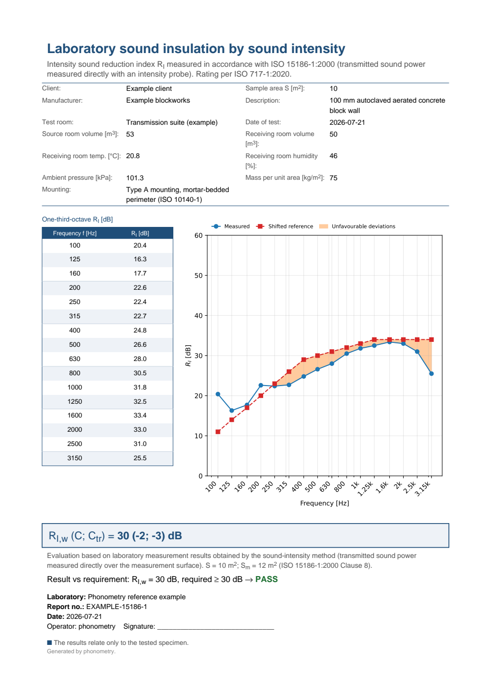
One-page laboratory intensity sound insulation test report of a building element: the metadata header (client, specimen description, mounting, sample area, room volumes, climate), the one-third-octave RI table beside the measured-versus-shifted-reference curve, the boxed RI,w (C; Ctr) rating evaluated per ISO 717-1, the intensity-method statement and a PASS verdict against the 30 dB requirement.
Small building elements: the element-normalized level difference
Section titled “Small building elements: the element-normalized level difference”For a small building element (a ventilator, a socket, a small window) the
intensity method reports the element-normalized level difference
(Formula (8)) instead, normalized to the reference absorption area
. IntensityElementNormalizedResult.report() writes the
same one-page fiche through the shared renderer, boxing DI,n,e,w (C; Ctr)
rated per ISO 717-1; verbose=True shows the ISO 717 evaluation per band and a
requirement adds a PASS/FAIL verdict (the element insulation passes at or
above the target).
import numpy as npfrom phonometry import building, ReportMetadata
lp1, sm, n = 85.0, 12.0, 1                              # source SPL, surface, unitsl_in = np.array([57.9, 62.0, 60.6, 55.7, 55.9, 55.6, 53.5, 51.7,                 50.3, 47.8, 46.5, 45.8, 44.9, 45.3, 47.3, 52.8])res = building.intensity_element_normalized_difference(    np.full(16, lp1), l_in, measurement_area=sm, n=n)res.plot()   # DI,n,e vs shifted ISO 717-1 reference (needs matplotlib)metadata = ReportMetadata(    specimen="Trickle ventilator in a 100 mm masonry wall",    measurement_standard="ISO 15186-1",    laboratory="Phonometry Reference Laboratory",    report_id="PHN-2026-0151",    requirement=30.0,                                   # DI,n,e,w >= 30 dB -> PASS)res.report("DIne.pdf", metadata=metadata)               # DI,n,e,w (C; Ctr)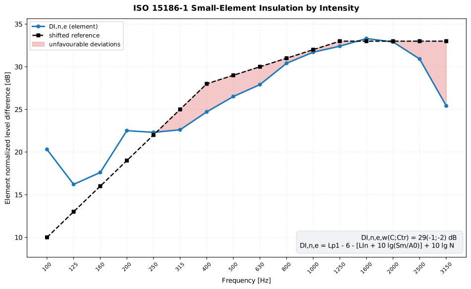
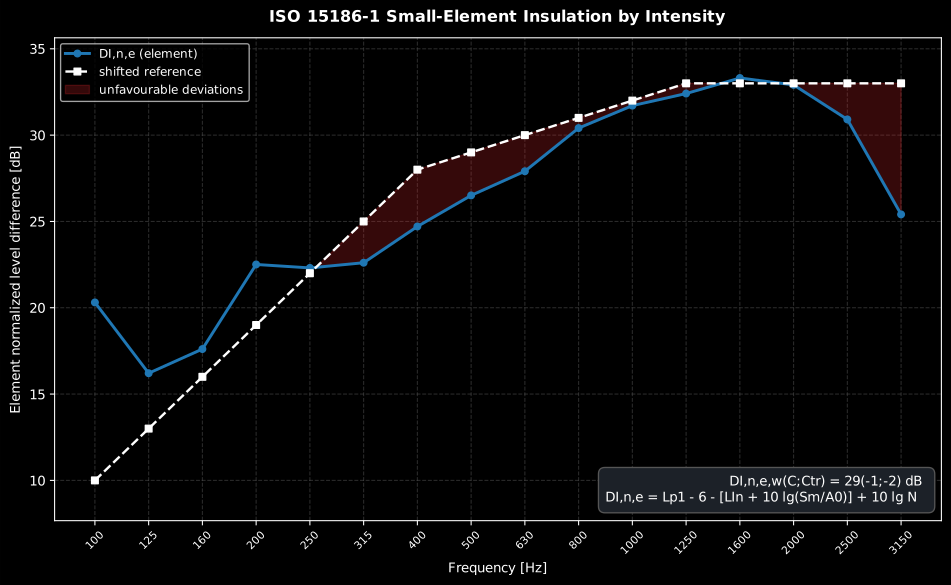
The small element is rated exactly like a wall: feeds the ISO 717-1 engine and the unfavourable deviations (reference above the measurement) set . The normalization replaces the specimen-area term, so the number describes the element irrespective of the wall it sits in.
Show the code for this figure
import matplotlib.pyplot as pltimport numpy as npfrom phonometry import building
# A trickle ventilator in a masonry wall: source-room SPL 85 dB and the# normal intensity level over the Sm = 12 m2 measurement surface.l_in = np.array([57.9, 62.0, 60.6, 55.7, 55.9, 55.6, 53.5, 51.7,                 50.3, 47.8, 46.5, 45.8, 44.9, 45.3, 47.3, 52.8])res = building.intensity_element_normalized_difference(    np.full(16, 85.0), l_in, measurement_area=12.0, n=1)
# One line — DI,n,e vs the shifted ISO 717-1 reference:res.plot()plt.show()
# By hand, from the rating the result carries:w = res.ratingfig, ax = plt.subplots()ax.semilogx(w.band_centers, res.d_i_n_e, "o-", label="DI,n,e (element)")ax.semilogx(w.band_centers, w.shifted_reference, "s--",            label="shifted reference")ax.fill_between(w.band_centers, w.measured, w.shifted_reference,                where=w.measured < w.shifted_reference, interpolate=True,                alpha=0.3, label="unfavourable deviations")ax.set_xlabel("Frequency [Hz]")ax.set_ylabel("Element normalized level difference [dB]")ax.set_title(f"DI,n,e,w = {w.rating} dB  (C={w.c:+d}; Ctr={w.ctr:+d})")ax.legend()plt.show()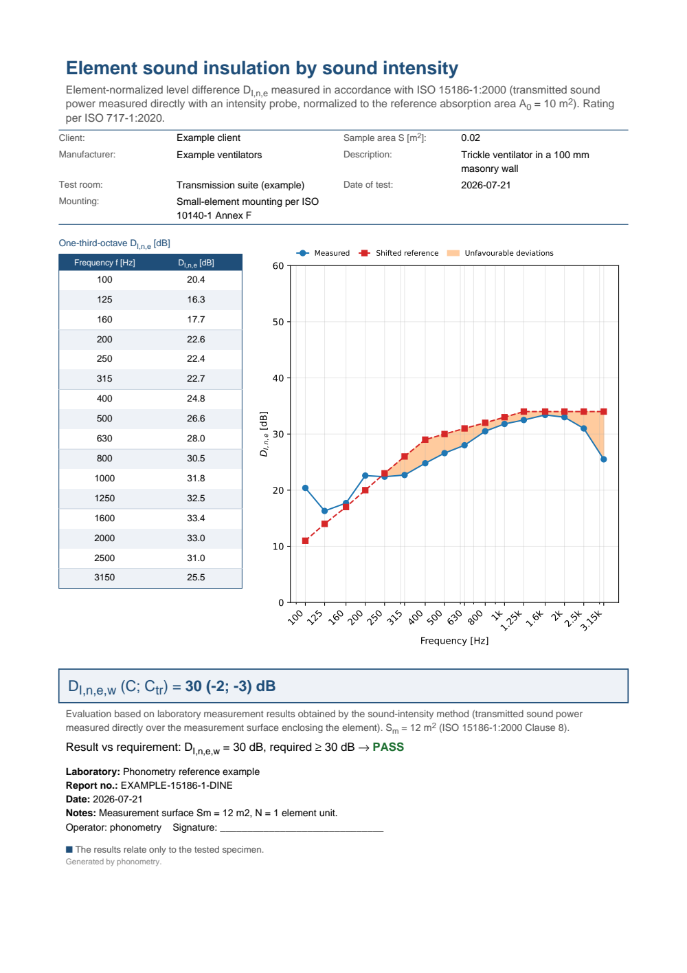
One-page laboratory element-normalized sound intensity insulation test report of a small building element: the metadata header (client, specimen description, mounting, element area), the one-third-octave DI,n,e table beside the measured-versus-shifted-reference curve, the boxed DI,n,e,w (C; Ctr) rating evaluated per ISO 717-1, the intensity-method statement and a PASS verdict against the 30 dB requirement.
Laboratory or field (ISO 15186-2)
Section titled “Laboratory or field (ISO 15186-2)”Part 1 is a laboratory method: the specimen sits in a test opening between two rooms, and the suppressed flanking of the facility makes a property of the element. ISO 15186-2 takes the same probe, the same surface scan and the same formula into the finished building, where the result is the apparent index of the installed element, flanking radiation and all. The selectivity that motivated the method in the laboratory doubles in the field: because the probe reads only what its measurement surface radiates, partial surfaces isolate which element (the wall itself, a window, a leaky junction) carries the transmitted power, which no pressure-based field method can resolve. Qualify each scan with the same pressure-intensity indicator, and expect the probe’s own limits (the spacer phase error) to set the usable low-frequency range.
Low frequencies: the pressure on the specimen (ISO 15186-3)
Section titled “Low frequencies: the pressure on the specimen (ISO 15186-3)”Both parts above put the source microphone in the room, and below 100 Hz that is exactly where a source room stops being able to answer. A room a laboratory can build has too few modes down there for a space average to describe the field driving the specimen: move the microphones and the average moves with them. ISO 15186-3 keeps the intensity probe on the receiving side and changes the other end of the measurement: the source-room level is read on the surface of the test specimen itself, from fixed microphones no more than 50 mm from it (Clause 6.3):
Nine decibels, not six. That single constant is the whole difference from Part 1. Close to a rigid boundary a diffuse field carries twice the mean-square pressure it carries away from one, so a microphone 50 mm from the specimen reads 3 dB above the room average of the same field. Part 1’s room average carries no such build-up and subtracts 6; the surface average carries it and subtracts 9. Everything else in the formula (the measurement-surface area ratio, the sign of the intensity, the subarea combination) is the method you already have.
The price is a validity condition Part 1 does not have. The doubling is only 3 dB if the surface reflects, so a NOTE under Formula (7) restricts it: the formula holds for a specimen with a reflecting surface in the source room, still works for moderately absorbing ones (100 mm of porous absorber), should be read only from 50 Hz to 80 Hz behind 100 mm to 200 mm of absorber, and is not valid behind anything thicker. Nothing in the library can see the specimen, so this one is on you.
How many microphones (Clause 6.3). Distributed evenly but asymmetrically over the whole surface, edges and corners included, at least 30 s of integration each:
| Test specimen | Minimum fixed microphone positions |
|---|---|
| Small building elements (ISO 140-10) | 2 for each element mounted in the test wall |
| Other elements up to 3 m² | 6 |
| Others | 12 |
The bands. Clause 6.6 requires filters at 50 Hz, 63 Hz and 80 Hz and allows 100 Hz, 125 Hz and 160 Hz to be added; the ceiling itself is Clause 1.1’s, which applies this part over 50 Hz to 160 Hz and says it is mainly intended for 50 Hz to 80 Hz. Six bands is the whole method, which is why no single-number rating comes out of it; ISO 717-1 needs sixteen. Passing a band outside that range is refused rather than extrapolated, and Clause 1.1 says what to do instead: combine these results with ISO 140-3 and ISO 15186-1 into one curve over 50 Hz to 5000 Hz.
Qualifying the surface (Clause 6.4.2). The indicator is the same as everywhere else in the series, and both of its levels are read on the measurement surface in the receiving room; it is not the surface level Formula (7) is built from. The limits distinguish the specimen, not the room: dB refuses a sound-reflecting specimen and dB one that presents a sound-absorbing surface in the receiving room, which is the two-absorbing-sides case, since a specimen absorbing on one side is mounted with that side towards the source (Clause 5.3). The receiving room always has an efficient absorber on the wall opposite the specimen; that is a facility requirement, not a case. Clause 6.5 adds the 10 dB background margin and its own test: with dB, drop the source by 10 dB, and if moves by less than 1 dB the requirement is met.
Because the standard only asks for that second pressure measurement “if
possible”, l_p is optional here. Without it there is no indicator and no
verdict, and the result says so rather than guessing:
import numpy as npfrom phonometry import building
# A light partition, 10 m2, scanned over a 12.6 m2 box surface. LpS is the# average over the surface of the specimen in the source room; LIn and Lp are# read together on the measurement surface in the receiving room.freqs = [50.0, 63.0, 80.0, 100.0, 125.0, 160.0]lp_surface = np.array([88.4, 89.1, 90.3, 91.0, 91.4, 91.8])l_in = np.array([61.6, 60.9, 59.8, 57.9, 56.0, 53.9])l_p = np.array([74.0, 72.0, 69.4, 66.1, 63.1, 60.3])
res = building.low_frequency_intensity_reduction(    lp_surface, l_in, measurement_area=12.6, area=10.0,    l_p=l_p, frequencies=freqs,)print(np.round(res.r_i, 1))                       # [16.8 18.2 20.5 23.1 25.4 27.9]print(np.round(res.surface_pressure_intensity_indicator, 1))  # [12.4 11.1  9.6  8.2  7.1  6.4]print(res.qualified.tolist())   # [False, False, True, True, True, True]print(res.indicator_limit)      # 10.0
# Without the receiving-side pressure there is no Clause 6.4.2 answer at all.bare = building.low_frequency_intensity_reduction(    lp_surface, l_in, measurement_area=12.6, area=10.0, frequencies=freqs,)print(bare.surface_pressure_intensity_indicator, bare.qualified)   # None None
A refused band is flagged, not dropped. The standard’s answer to over the limit is to improve the measurement environment: increase the measurement distance by 5 cm to 10 cm first, then reduce flanking or improve the absorber opposite. That is why the index is still computed and the verdict travels beside it.
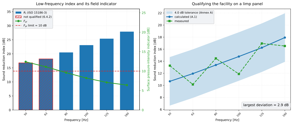
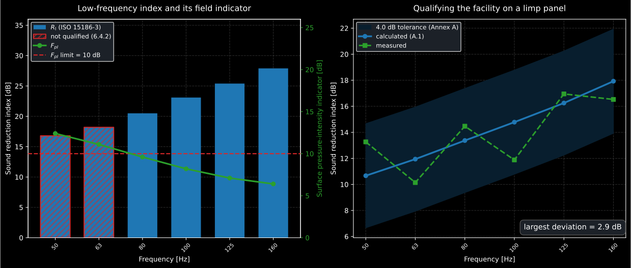
Left, the measurement: the index rises through the six bands while the indicator falls past its limit, so the two lowest bands are computed but not qualified. Right, the facility: Annex A’s calculated limp-panel curve and the 4 dB either side of it that a measurement has to stay within.
Show the code for this figure
import matplotlib.pyplot as plt
# res is the LowFrequencyIntensityResult computed above. One line:res.plot()   # RI bars, refused bands hatched, FpI and its limit on a twin axisplt.show()
# By hand, and the Annex A panel beside it.calculated = building.limp_panel_reduction_index(    freqs, surface_mass=10.0, area=10.0, temperature_c=23.0,)measured = calculated + np.array([2.6, -1.8, 1.1, -2.9, 0.7, -1.4])x = np.arange(len(freqs))fig, (axl, axr) = plt.subplots(1, 2, figsize=(13.0, 5.6))bars = axl.bar(x, res.r_i, width=0.68)for bar, ok in zip(bars, res.qualified, strict=True):    if not ok:        bar.set_hatch("///")axl.set_xticks(x, [f"{f:g}" for f in freqs])axl.set(xlabel="Frequency [Hz]", ylabel="Sound reduction index [dB]")twin = axl.twinx()twin.plot(x, res.surface_pressure_intensity_indicator, "-o", color="#2ca02c", label="FpI")twin.axhline(res.indicator_limit, ls="--", color="#d62728", label="FpI limit")twin.set_ylabel("Surface pressure-intensity indicator [dB]")twin.legend()axr.fill_between(x, calculated - 4.0, calculated + 4.0, alpha=0.2,                 label="4.0 dB tolerance (Annex A)")axr.plot(x, calculated, "-o", label="calculated (A.1)")axr.plot(x, measured, "--s", label="measured")axr.set_xticks(x, [f"{f:g}" for f in freqs])axr.set(xlabel="Frequency [Hz]", ylabel="Sound reduction index [dB]")axr.legend()plt.show()
Small elements at low frequencies, and a sign the series disagrees on
Section titled “Small elements at low frequencies, and a sign the series disagrees on”Formula (8) normalizes a small element to the reference absorption area m² exactly as Part 1 does, with the 9 dB of the surface measurement in place of 6:
Read the bracket carefully. The inside it is subtracted, so the term reaches added, which is the sign this library derives, and the opposite of what ISO 15186-1 prints for the same quantity. Two parts of one series print the two signs; this is the one that agrees with the physics (installing units raises the transmitted power by , so recovering the per-unit figure has to add it back) and with the pressure-based ISO 10140-2 Formula (6). The Part 1 print is registered in ERRATA, and Part 1’s implementation warns whenever puts it at odds with its own page. Nothing warns here, because here the page and the physics agree.
# Four identical trickle ventilators inside one 2.0 m2 measurement surface.element = building.low_frequency_element_normalized_difference( np.full(6, 90.0), np.array([62.0, 61.0, 60.0, 58.0, 57.0, 55.0]), measurement_area=2.0, elements=4, frequencies=freqs,)print(np.round(element.d_i_n_e, 1)) # [32. 33. 34. 36. 37. 39.]print(element.elements) # 4Qualifying the facility (Annex A)
Section titled “Qualifying the facility (Annex A)”Annex A is normative, and it is what a laboratory does before it reports anything: measure a limp panel of more than 1 m², calculate what it should read, and require the two to agree within 4,0 dB from 50 Hz to 160 Hz. The calculated half is forced transmission and nothing else: mass law reduced by the radiation efficiency of a plate driven by a diffuse field:
with the air taken at the climate of the test, and . The panel is limp by assumption. The 160 Hz ceiling is not the annex’s own: Clause 1.1 applies the whole of this part over 50 Hz to 160 Hz, and says it is mainly intended for 50 Hz to 80 Hz.
# Annex A, Table A.1: 12,5 mm plaster board, 10 kg/m2, over a 10 m2 opening,# at 1 013 hPa and 23 degC.calc = building.limp_panel_reduction_index( freqs, surface_mass=10.0, area=10.0, temperature_c=23.0, static_pressure_pa=101300.0,)print(np.round(calc, 1)) # [10.7 11.9 13.4 14.8 16.3 17.9]Those six values are the printed table, band for band, and they are the conformance anchor for all five formulas. The steel-sandwich column beside them in the same table is not: no reading of the inputs printed next to it reproduces it, and the one that would takes an area and a surface mass moved together, the mass landing heavier than solid steel of the stated thickness. It is registered in ERRATA and is deliberately not used as an oracle.
low_frequency_intensity_reduction(), low_frequency_element_normalized_difference() and limp_panel_reduction_index() parameters
Section titled “low_frequency_intensity_reduction(), low_frequency_element_normalized_difference() and limp_panel_reduction_index() parameters”| Parameter | Type | Units | Range / default | Notes |
|---|---|---|---|---|
lp_surface | 1D or 2D array | dB | one/band, or (positions, bands) | Pressure over the surface of the specimen, |
l_in | 1D or 2D array | dB | one/band, or (positions, bands) | Normal intensity level over the measurement surface |
measurement_area | float | m² | > 0 | Measurement-surface area |
area | float | m² | > 0 | Specimen area ; the limp panel of Annex A needs m² |
l_p | 1D or 2D array | dB | one/band / None | Receiving-side pressure on the measurement surface, for Formula (5) |
frequencies | 1D array | Hz | 50 to 160 / None | Mid-band frequencies; Clause 6.6 admits no others |
absorbing_specimen_surface | bool | — | default False | True tightens the Clause 6.4.2 limit to 6 dB |
elements | int | element units | ≥ 1, default 1 | Number of units (low_frequency_element_normalized_difference only) |
surface_mass | float | kg/m² | > 0 | Limp-panel surface mass (limp_panel_reduction_index) |
temperature_c / static_pressure_pa | float | °C / Pa | default 23 °C, 101 300 Pa | The climate of Formulas (A.4) and (A.5) |
low_frequency_intensity_reduction() returns a LowFrequencyIntensityResult
(r_i, surface_pressure_intensity_indicator, qualified,
indicator_limit), low_frequency_element_normalized_difference() a
LowFrequencyElementResult (d_i_n_e and the same three), and
limp_panel_reduction_index() a plain array. Neither result carries a rating:
Clause 7 asks for the index to one decimal beside the indicator, and six bands
cannot feed ISO 717-1.
What this guide covers
Section titled “What this guide covers”Covered
ISO 15186-1:2000’s intensity sound reduction index (Clause 3.8), its -modified (Annex B) and the element-normalized (Clause 3.9), with the subarea combination of Formulas (11)-(12) and the surface pressure-intensity indicator, via
building.intensity_sound_reduction,building.adaptation_term_kc,building.intensity_element_normalized_difference,building.surface_pressure_intensity_indicatorandbuilding.combine_subareas; the single-number ratings reuse the verified ISO 717-1 engine, and both results write the one-page test fiche through.report(). ISO 15186-3:2002’s low-frequency variant is covered too: the surface-pressure index of Formula (7), the element-normalized of Formula (8), the Clause 6.4.2 qualification against both of its limits, the Clause 6.6 band range and the normative limp-panel qualification of Annex A, viabuilding.low_frequency_intensity_reduction,building.low_frequency_element_normalized_differenceandbuilding.limp_panel_reduction_index.Not covered
The sound-intensity measurement itself (the scanning probe, the two-microphone acquisition and phase-mismatch calibration behind and ) is not implemented: both levels are taken as already-measured inputs, and the ISO 15186-1 report fiche states explicitly that it has no field for the measurement-surface geometry or the scanning-versus-discrete-point acquisition method. Nothing here enforces the Clause 6.4 acquisition documented above either (the 0.1–0.3 m stand-off, the 0.1–0.3 m/s scan speed, the 90°-rotated second scan and its 1.0 dB validity test, the 10 dB background margin), so a single scan will produce a number just as readily as a qualified pair. ISO 15186-2’s own field procedure (loudspeaker positions, the façade cases) is not implemented either: the formulas here apply unchanged to field data, but nothing checks how that data was acquired. The same holds of Part 3’s procedure: the microphone counts of its Table 1, the 50 mm stand-off, the two 90°-rotated scans and their 2,0 dB / 1,0 dB agreement test, the 10 dB background margin and the source-room absorption limits under Formula (7) are documented above and enforced nowhere. Part 3 results carry no single-number rating and no
.report()fiche, because six bands cannot feed ISO 717-1 and the standard’s Clause 8 report has no worked form here.
References
Section titled “References”- Hopkins, C. (2007). Sound insulation. Butterworth-Heinemann. https://doi.org/10.4324/9780080550473The reference monograph for laboratory sound-insulation measurement, including the intensity route and its relation to the pressure methods. ISBN 978-0-7506-6526-1.
- International Organization for Standardization. (2000). Acoustics — Measurement of sound insulation in buildings and of building elements using sound intensity — Part 1: Laboratory measurements (ISO 15186-1:2000). The sound-intensity sound reduction index R_I, its Kc-modified form and the element normalized level difference (laboratory); the tool of choice when flanking is high (Clause 1).
- International Organization for Standardization. (2002). Acoustics — Measurement of sound insulation in buildings and of building elements using sound intensity — Part 3: Laboratory measurements at low frequencies (ISO 15186-3:2002). The low-frequency variant: the source-room level is read on the surface of the specimen and 9 dB is subtracted instead of 6 (Clause 3.8), with the normative limp-panel qualification of Annex A.
- International Organization for Standardization. (2003). Acoustics — Measurement of sound insulation in buildings and of building elements using sound intensity — Part 2: Field measurements (ISO 15186-2:2003). The field counterpart of the intensity method, giving the apparent index R'_I.