Image Sources and the Steady-State Room Field

Key references: Kuttruff 2016 Vorländer 2020 Allen & Berkley 1979 Bies et al. 2017 Long 2014

Two classical models predict the sound field in a rectangular room before it is ever built. The image-source model gives the deterministic early reflection pattern — the whole room impulse response as a sum of mirror images of the source — while the steady-state model gives the statistical level a source of known power settles to, split into a direct and a reverberant field. This page covers both in phonometry.room: the first complements the measured impulse response of the Room Acoustics guide with a synthetic one, and the second complements the single decay rate of the Reverberation-time prediction guide with a level-versus-distance prediction, bridging the sound power of a source and the level it produces indoors.

1. Image-source room impulse response

A rigid or absorbing rectangular room — a shoebox — reflects a point source in its six walls, and each reflection is exactly the free-field sound of a mirror image of the source. Mirroring a coordinate in a wall ( $S_{n} = S - 2 d n$ ) turns the source into a regular lattice of images, and the room impulse response is the direct sound plus one delayed, attenuated impulse per image,

g (t) = n \sum A_{n} δ (t - t_{n}), A_{n} = \frac{1}{4 π r _{n}} e^{- m r_{n} /2} walls \prod R_{w}^{k_{w, n}}, t_{n} = \frac{r _{n}}{c} .

Each image at distance $r_{n}$ from the receiver arrives at $t_{n} = r_{n} / c$ with an amplitude built from the $1/ (4 π r_{n})$ spherical spreading, the product of the wall pressure reflection factors $R_{w} = 1 - α_{w}$ each raised to the number of reflections $k_{w, n}$ that image made off wall $w$ , and the air pressure loss $e^{- m r_{n} /2}$ over the path ( $m$ the power (intensity) attenuation coefficient in neper per metre, so intensity falls as $e^{- m r}$ and pressure as $e^{- m r /2}$ — the same $m$ the reverberation-time and EN 12354-6 guides feed to their $4 mV$ terms). A shoebox has exactly $\frac{2}{3} (2 i_{0}^{3} + 3 i_{0}^{2} + 4 i_{0})$ audible images up to reflection order $i_{0}$ (1560 at order 10), and the reflection density grows as $d N / d t = 4 π c^{3} t^{2} / V$ .

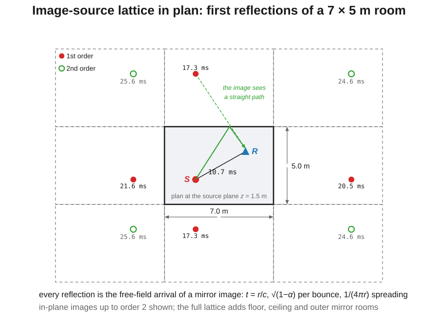
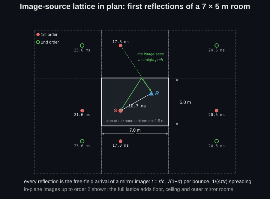
The construction in one plan: every wall reflection is the straight-line sound of an image in a mirror room, so the geometry alone fixes each arrival. In the 7 × 5 m room below the direct sound lands at 10.7 ms and the four first-order lateral images in plan follow between 17.3 and 21.6 ms; the ceiling and floor images of the 3-D room are omitted from the drawing.

Plan of a 7 by 5 m room in the centre of its three by three grid of dashed mirror rooms: the source at (2, 1.6) and the receiver at (5.2, 3.4) joined by the 10.7 ms direct sound, filled first-order images in the four adjacent rooms labelled with their arrival times of 17.3, 20.5 and 21.6 ms, outlined second-order images in the corner rooms at 24.6 and 25.6 ms, and the first far-wall reflection drawn twice, as the real bent path off the wall and as the straight dashed line from the image to the receiver

import numpy as np
from phonometry import room

# A 7 x 5 x 3 m room, source and receiver off-centre.
res = room.image_source_rir(
    dimensions=(7.0, 5.0, 3.0),
    source=(2.0, 1.6, 1.5),
    receiver=(5.2, 3.4, 1.7),
    absorption=0.12,          # uniform wall absorption (scalar)
    fs=48000,
    # Enough order to cover a T30 fit; see "Choosing max_order, duration and
    # fs" below. The default 20 truncates this room's tail by half.
    max_order=60,
)

print(res.ir.shape)                          # (n_samples,) broadband RIR
print(round(res.direct_time * 1000, 2))      # 10.72  direct-sound arrival, ms
print(res.times.size == room.audible_image_count(60) + 1)   # images + source

res.plot()   # the reflectogram; the figure below draws the same room at order 10

# The synthetic RIR flows straight into the ISO 3382 decay analysis.
params = room.room_parameters(res.ir, res.fs, limits=None)
print(bool(params.t30_valid[0]))             # True: the decay window is usable
print(round(float(params.t30[0]), 2))        # 1.06 s, specular
print(round(float(room.eyring_reverberation_time(105.0, [(142.0, 0.12)])), 2))
# 0.93 s, the diffuse-field Eyring estimate for the same room

image_source_rir returns an ImageSourceResult. Its ir is the sampled RIR (a 1D array broadband, or one row per octave band for per-band absorption), while the exact sub-sample reflection table stays in times, distances, orders, amplitudes and image_positions — so the geometry is exact regardless of the sample rate. The direct sound and the individual early reflections are geometric quantities good to machine precision.

Read as a list of arrivals, that table hides what the method actually is. Each image sits at a fixed distance $r_{n}$ from the receiver and contributes one arrival at $r_{n} / c$ , so the echogram is not a signal that decays — it is a static lattice of points being read off by a sphere expanding from the receiver at the speed of sound. That view turns the reflection density into something watchable: the sphere’s volume grows as $t^{3}$ , the lattice has one image per room volume $V$ , and the count it has swept must therefore follow $N (t) = \frac{4 π}{3} (c t)^{3} / V$ , whose derivative is the $4 π c^{3} t^{2} / V$ reflection density quoted below. The clip sweeps it:

Download the animation (WebM)

The echogram is a lattice being swept, not a decaying signal. Because the expanding sphere gains volume as the cube of time while the images are spaced one per room volume, arrivals accumulate as the cube of time and their rate grows as its square — the early discrete reflections and the late diffuse tail are the same construction read at two densities.

Download the animation (WebM)

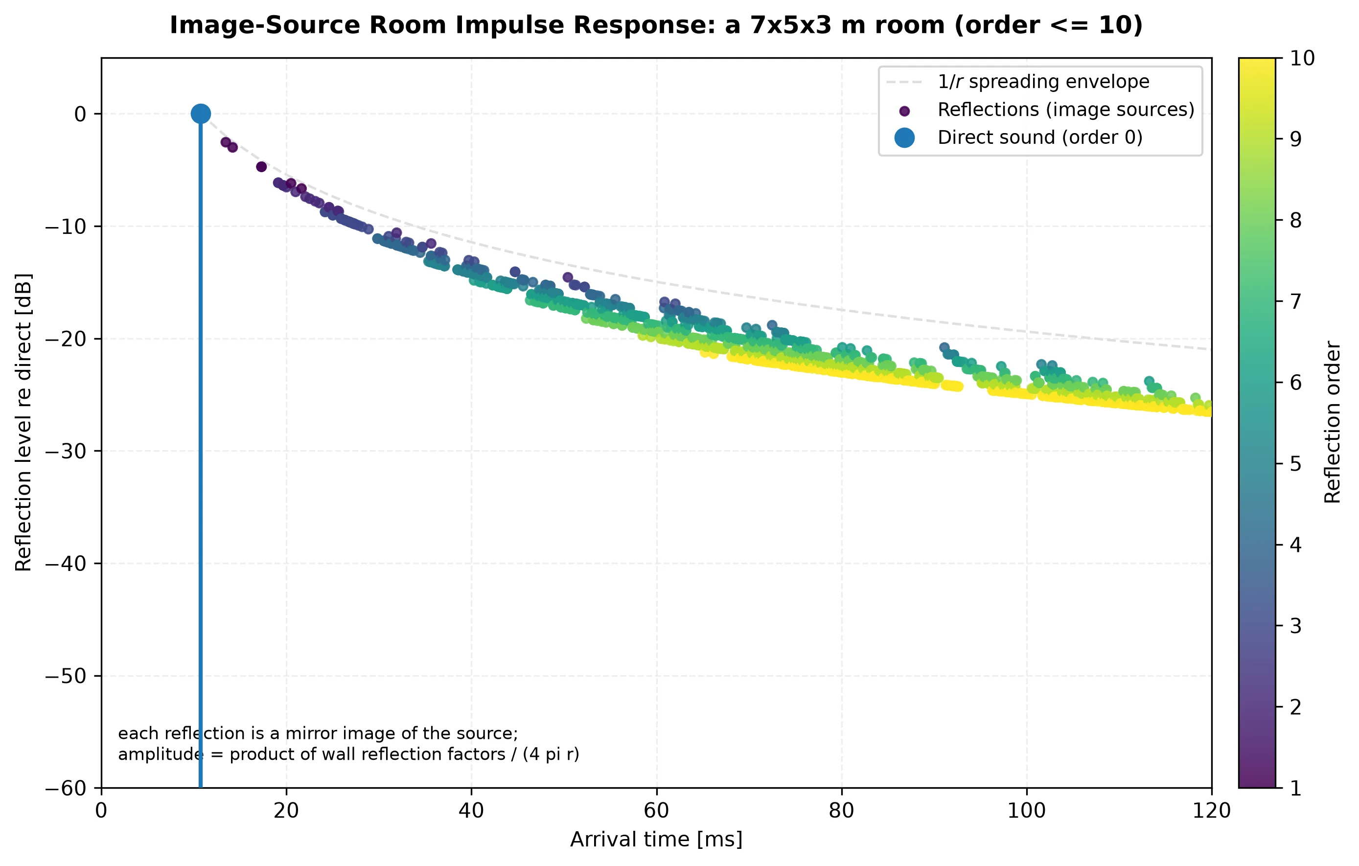
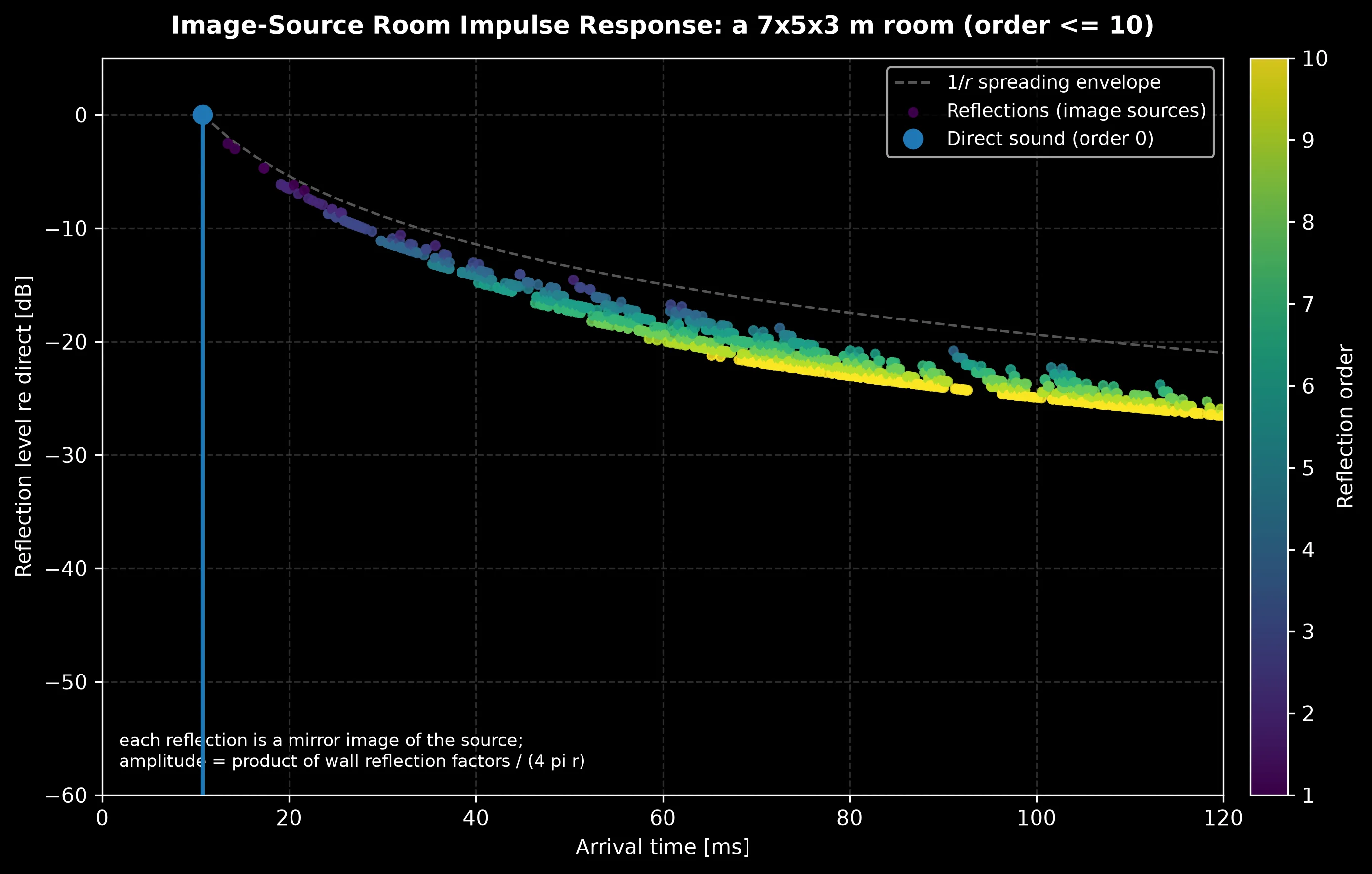
The reflectogram below shows the whole pattern: the direct sound at 0 dB, then the reflection cloud coloured by reflection order decaying under the $1/ r$ spreading envelope. Order-1 reflections (the six walls) sit just below the direct sound; higher orders arrive later, denser and weaker.

Image-source reflectogram of a 7 by 5 by 3 metre room: the direct sound at 0 dB followed by a cloud of reflections coloured by reflection order that decays under the 1/r spreading envelope, denser and weaker with time

Show the code for this figure

import matplotlib.pyplot as plt
import numpy as np
from phonometry import room

res = room.image_source_rir((7.0, 5.0, 3.0), (2.0, 1.6, 1.5),
                            (5.2, 3.4, 1.7), 0.12, fs=48000, max_order=10)

# One line: the reflectogram (level in dB re direct vs arrival time, by order).
res.plot()
plt.show()

# By hand: scatter the reflection amplitudes coloured by order.
t_ms = np.asarray(res.times) * 1e3
amp = np.asarray(res.amplitudes)
level = 20 * np.log10(np.abs(amp) / np.max(np.abs(amp)))
order = np.asarray(res.orders)
fig, ax = plt.subplots()
sc = ax.scatter(t_ms[order > 0], level[order > 0], c=order[order > 0],
                cmap="viridis", s=18)
ax.stem([t_ms[order == 0][0]], [0.0])         # direct sound
fig.colorbar(sc, label="Reflection order")
ax.set_xlabel("Arrival time [ms]"); ax.set_ylabel("Level re direct [dB]")
ax.set_xlim(0, 120); ax.set_ylim(-60, 5)
plt.show()

Every dot of the reflectogram is a mirror image at a definite place, and .plot_geometry() shows where: the plan view below draws the room, the source, the receiver and every image up to third order on the mirror-room grid, coloured by reflection order.

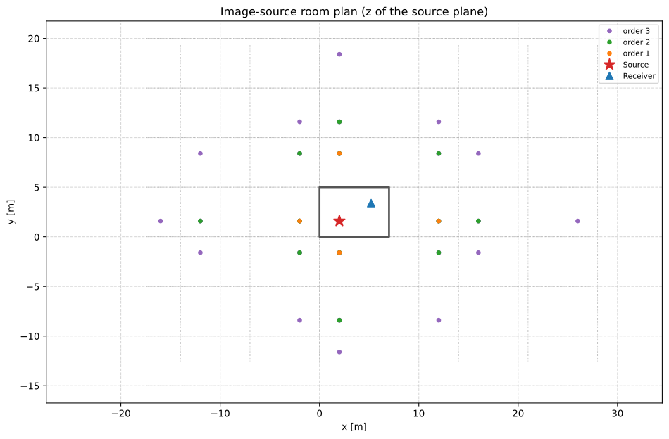
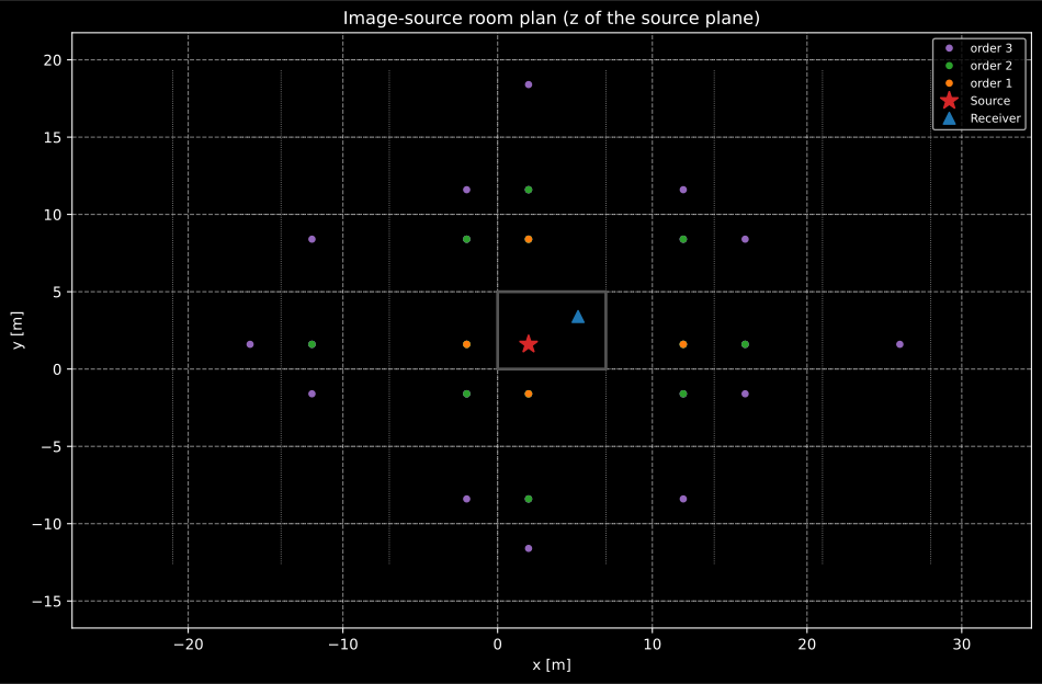
The same room, source and receiver as the reflectogram above, drawn to third order so the lattice stays legible — the reflectogram runs to order 10 and this plan is its first three shells. Each image sits in a mirror room at the height plane of the source, and its distance to the receiver alone fixes the arrival time and the $1/ (4 π r)$ spreading of that reflection.

Show the code for this figure

import matplotlib.pyplot as plt
from phonometry import room

res = room.image_source_rir((7.0, 5.0, 3.0), (2.0, 1.6, 1.5),
                            (5.2, 3.4, 1.7), 0.12, fs=48000, max_order=3)

# One line: the image lattice in plan, coloured by reflection order.
res.plot_geometry()
plt.show()

Per band, per wall and with air. Pass per-band coefficients (a (6, n_bands) per-wall array, a per-band vector or a frequencies list) to synthesise one decay per octave band; a length-6 vector sets each wall separately (order x0, xL, y0, yL, z0, zL); and air_attenuation (the intensity coefficient m from air_attenuation_m) adds the exp(-m r / 2) air loss that eats the high-frequency tail.

import numpy as np
from phonometry import room

freqs = [250.0, 500.0, 1000.0, 2000.0, 4000.0]
alpha = np.array([[0.10, 0.15, 0.25, 0.40, 0.50]] * 6)   # (6 walls, 5 bands)
res = room.image_source_rir((7.0, 5.0, 3.0), (2.0, 1.6, 1.5), (5.2, 3.4, 1.7),
                            alpha, fs=48000, max_order=60, frequencies=freqs)
print(res.ir.shape)                                  # (5 bands, n_samples)
res.plot()   # one decay per band; the figure below adds the air term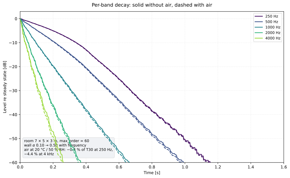

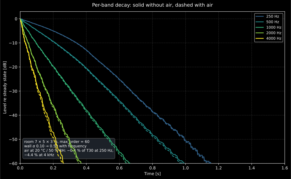
Schroeder decay curves of the five octave bands of a 7 by 5 by 3 metre room, each band drawn twice: solid without air attenuation and dashed with the coefficient m at 20 degrees Celsius and 50 per cent relative humidity. The bands fan out from a 1.06 second decay at 250 hertz to 0.25 seconds at 4 kilohertz, and each dashed curve sits only slightly below its solid partner, the gap widening with frequency

The banded branch of image_source_rir for the page’s own room, each band drawn without air (solid) and with $m$ at 20 °C / 50 % RH (dashed). The bands fan out because the wall absorption rises with frequency, from T30 = 1.06 s at 250 Hz to 0.25 s at 4 kHz. The air term is the second, much smaller mechanism here: it takes 0.4 % off the 250 Hz decay and 4.4 % off the 4 kHz decay. That is the honest size of the effect in a 105 m³ room — the reflections simply do not travel far enough — and it is why air absorption is a volume effect rather than a frequency effect: put the same walls around 2 000 m³ and the same argument takes tens of per cent off the top band.

Show the code for this figure

import matplotlib.pyplot as plt
# `np`, `room`, `freqs` and `alpha` come from the per-band block above.

# environment.air_attenuation_m(freqs, 20.0, 50.0), Np/m at 20 C / 50 % RH
m = [3.02e-4, 6.28e-4, 1.074e-3, 2.277e-3, 6.831e-3]

fig, ax = plt.subplots()
for attenuation, style in ((0.0, "-"), (m, "--")):
    banded = room.image_source_rir(
        (7.0, 5.0, 3.0), (2.0, 1.6, 1.5), (5.2, 3.4, 1.7), alpha,
        fs=48000, max_order=60, frequencies=freqs,
        air_attenuation=attenuation,
    )
    for row, f in zip(banded.ir, freqs):
        time, level = room.decay_curve(row, banded.fs)
        ax.plot(time, level, style, label=f"{f:g} Hz")
ax.set_xlabel("Time [s]")
ax.set_ylabel("Level re steady state [dB]")
plt.show()

Reproducing the statistical decay. The initial decay rate of the synthetic RIR reproduces the Eyring reverberation time $T = - 24 V ln 10/ (c S ln (1 - \overset{α}{ˉ}))$ , because the mean reflection rate $c S /4 V$ equals $\frac{c}{2} (1/ L_{x} + 1/ L_{y} + 1/ L_{z})$ . The match is close only in the near-cubic limit: an elongated room sustains energy along its long axis, so its pure specular decay runs slower than the diffuse-field Eyring estimate — exactly the anisotropy the Fitzroy and Arau-Puchades models were built to correct. The model captures specular reflections only (no diffraction, no diffuse scattering) and is exact for real, angle-independent wall reflection factors.

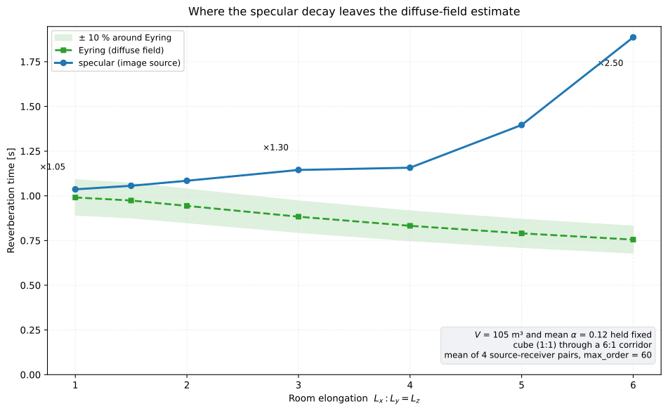
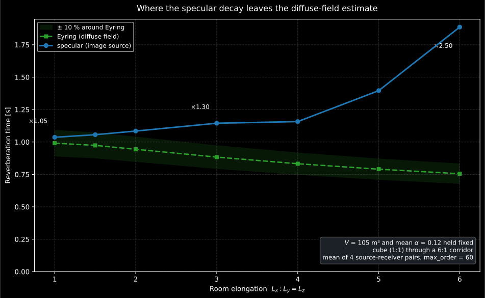
Specular initial-decay time against room elongation at constant volume and constant mean absorption: the Eyring prediction falls slowly as the room is stretched while the specular decay rises, so the ratio between them grows from 1.05 at a cube to about 2.5 at a six to one corridor, leaving the shaded plus or minus 10 per cent band around Eyring at an elongation of roughly 1.5 to 1

The same 105 m³ and the same uniform $\overset{α}{ˉ}$ = 0.12, stretched from a cube to a 6:1 corridor. Eyring falls as the room is stretched, because stretching at constant volume adds boundary area; the specular decay rises, because the long axis keeps returning energy that the mean free path has already written off. The two agree to 5 % for the cube — the documented tolerance of the Validation section below — and part company immediately: past about 1.5:1 the specular decay is outside the ±10 % band, and at 6:1 it is 2.5 times the Eyring estimate. This is the anisotropy that motivates the Fitzroy and Arau-Puchades models, and the reason the reverberation-prediction guide lists disproportionate rooms among the cases where every statistical formula fails.

Show the code for this figure

import matplotlib.pyplot as plt
# `np` and `room` are the imports of the per-band block above.

volume, alpha = 105.0, 0.12
side = volume ** (1.0 / 3.0)
ratios, specular, eyring = [1.0, 1.5, 2.0, 3.0, 4.0, 5.0, 6.0], [], []
for r in ratios:
    lx, ly = side * r ** (2.0 / 3.0), side * r ** (-1.0 / 3.0)
    area = 2.0 * (2.0 * lx * ly + ly * ly)      # a box lx x ly x ly
    eyring.append(room.eyring_reverberation_time(volume, [(area, alpha)]))
    res = room.image_source_rir((lx, ly, ly), (lx * 0.28, ly * 0.32, ly * 0.5),
                                (lx * 0.74, ly * 0.68, ly * 0.57), alpha,
                                fs=48000, max_order=60)
    # The initial slope of the reverberant energy density, from the exact
    # reflection table rather than from the sampled IR.
    edges = np.arange(0.0, float(np.max(res.times)), 0.004)
    energy, _ = np.histogram(res.times, bins=edges, weights=np.asarray(res.amplitudes) ** 2)
    centres, good = 0.5 * (edges[:-1] + edges[1:]), energy > 0.0
    level = 10.0 * np.log10(np.where(good, energy, 1.0) / energy[good][0])
    band = good & (level <= -1.0) & (level >= -20.0)
    specular.append(-60.0 / np.polyfit(centres[band], level[band], 1)[0])

fig, ax = plt.subplots()
ax.plot(ratios, eyring, "--", label="Eyring")
ax.plot(ratios, specular, "-o", label="specular (image source)")
ax.set_xlabel("Room elongation $L_x : L_y = L_z$")
ax.set_ylabel("Reverberation time [s]")
ax.legend()
plt.show()

`image_source_rir()` parameters

Parameter	Type	Units	Range / default	Notes
`dimensions`	(float, float, float)	m	all > 0	Room lengths `(Lx, Ly, Lz)`
`source` / `receiver`	(float, float, float)	m	strictly inside the room	Positions `(x, y, z)`
`absorption`	scalar / (6,) / (n,) / (6, n)	—	`[0, 1]`	Uniform, per-wall, per-band, or per-wall per-band
`fs`	int	Hz	> 0	Sample rate
`max_order`	int	—	≥ 0, default 20	Reflection-order cut-off
`speed_of_sound`	float	m/s	> 0, default 343	Speed of sound `c`
`air_attenuation`	float or (n,)	1/m	≥ 0, default 0	Air intensity coefficient `m`
`duration`	float, optional	s	> 0	RIR length (default: last image arrival)
`frequencies`	(n,), optional	Hz	—	Band centres labelling a per-band result

Returns an ImageSourceResult (ir, fs, frequencies, and the exact times/distances/orders/amplitudes/image_positions reflection table) with .plot(), .plot_geometry() (the mirror-room plan above) and a direct_time property. audible_image_count(order) gives the shoebox image count and reflection_density(t, volume) the density $4 π c^{3} t^{2} / V$ .

Choosing `max_order`, `duration` and `fs`

max_order is not a quality knob, it is a time horizon. The image lattice is complete only out to a radius of roughly max_order × the shortest room dimension, so covering $t$ seconds of decay needs

order \approx \frac{c t}{L _{min}} .

A T30 fit spans 35 dB, about $0.58 T$ of decay. The 7 × 5 × 3 m room above has $L_{min} = 3$ m and an Eyring time near 0.93 s, so it needs $343 \times 0.54/3 \approx 60$ . Below that the tail is simply missing, and the fitted T30 comes out short:

`max_order`	audible images	fitted T30	runtime
12	2 624	0.28 s	< 0.1 s
20 (default)	11 520	0.43 s	< 0.1 s
30	37 880	0.60 s	< 0.1 s
40	88 640	0.75 s	0.1 s
60	295 360	1.06 s	0.2 s

The Eyring estimate for this room is 0.93 s, so order 12 is 3.3× short and the default 20 is 2.1× short. The cost objection does not apply: order 60 is 295 360 images and runs in a fifth of a second.

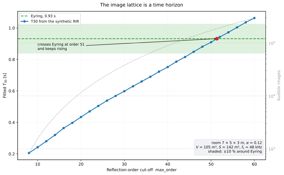
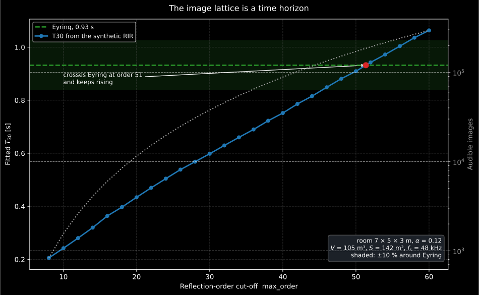
Fitted T30 and EDT of the 7 by 5 by 3 metre room against the reflection-order cut-off from 8 to 60: both rise steeply and almost linearly with order, T30 crossing the 0.93 second Eyring line and its shaded plus or minus 10 per cent band at about order 51 and continuing to rise, while a second axis shows the audible image count growing from about 800 to 295 thousand

T30 read by room_parameters from the synthetic RIR, against the order the lattice was built to. The rise is the truncation: every extra order adds a shell of later arrivals, so the fit window keeps finding more decay to fit. The completeness rule sets the floor — below the order that covers the fit window the number is simply wrong, which is what the table above quantifies — but it is not a convergence criterion. Past the crossing the specular T30 keeps drifting above Eyring, because a 7 × 5 × 3 room is not near-cubic and its long axis sustains energy the diffuse-field estimate has already spent; the next figure sweeps exactly that. Read T30 from this model as an order-dependent specular quantity, not as a prediction of a measured reverberation time.

Show the code for this figure

import matplotlib.pyplot as plt
# `room` is the import of the section 1 block above.

orders = list(range(8, 62, 2))
t30 = []
for order in orders:
    res = room.image_source_rir((7.0, 5.0, 3.0), (2.0, 1.6, 1.5),
                                (5.2, 3.4, 1.7), 0.12, fs=48000,
                                max_order=order)
    params = room.room_parameters(res.ir, res.fs, limits=None)
    t30.append(float(params.t30[0]))

eyring = float(room.eyring_reverberation_time(105.0, [(142.0, 0.12)]))
fig, ax = plt.subplots()
ax.plot(orders, t30, "-o", label="T30 from the synthetic RIR")
ax.axhline(eyring, ls="--", label=f"Eyring, {eyring:.2f} s")
ax.fill_between(orders, 0.9 * eyring, 1.1 * eyring, alpha=0.15)
ax.set_xlabel("max_order")
ax.set_ylabel("Reverberation time [s]")
ax.legend()
plt.show()

t30_valid cannot see a truncated lattice. It reads the decay range of whatever array it is handed, so it returns True at every order in the table above. The flag catches a noisy or too-short recording; it cannot catch a model that stopped generating reflections. A duration shorter than the decay truncates the tail exactly the same way, and silently.

Two more caveats belong to the same section. fs quantises every arrival to the sample grid, so early-reflection work — arrival times, ITDG, lateral fractions — should read the exact times / amplitudes table rather than peak-pick the sampled ir. And absorption enters as a real, angle-independent pressure reflection factor $1 - α$ , so grazing incidence is treated like normal incidence.

Finally, the honest boundary: if the order needed to cover the reverberation time makes the run impractical — a large room with a small $L_{min}$ , or a long tail — the pure image method is being asked to do a job that belongs to a hybrid model with a statistical late tail, or to the FDTD solver.

2. Steady-state room field

When a source of constant sound power runs in a room, the level settles to the sum of a direct field that falls with distance and a diffuse reverberant field that is (approximately) the same everywhere. The room constant $R = S \overset{α}{ˉ} / (1 - \overset{α}{ˉ})$ measures how much reverberant field a given power builds up, and the steady-state level is

L_{p} = L_{W} + 10 lo g_{10} (\frac{Q}{4 π r ^{2}} + \frac{4}{R}),

with the source directivity factor $Q$ (1 omnidirectional, 2 on a hard floor, 4 in an edge, 8 in a corner). The two terms cross at the critical distance $r_{c} = QR /16 π$ : closer than $r_{c}$ the direct field dominates and doubling the distance drops the level by 6 dB; farther out the reverberant field takes over and moving away barely helps.

The $(1 - \overset{α}{ˉ})$ in the denominator of $R$ and the 4 in the level equation come from the same bookkeeping. Only the power not absorbed at the first encounter goes on to build the reverberant field, which is what divides $A$ by $(1 - \overset{α}{ˉ})$ ; and the 4 is the diffuse-field factor between energy density and the intensity striking a surface — the same 4 as in the $4 mV$ air term of the reverberation formulae. That gives $R$ its reading: it is the area of open window that would remove power at the same rate, so a room with $R$ = 25 m² behaves, as far as a distant listener is concerned, like a room with 25 m² of open window. $R$ therefore always exceeds the Sabine area $A = S \overset{α}{ˉ}$ , and the difference vanishes as $\overset{α}{ˉ} \to 0$ , which is why the module prefers $R$ and why Kuttruff’s $A /16 π$ agrees with it in a live room.

Where a source is mounted is not a detail, because $Q$ moves $r_{c}$ as $Q$ : the same machine has a 1.11 m critical distance on a stand and a 3.14 m one in the corner of the same workshop. The plate below fixes the four values to real mountings.

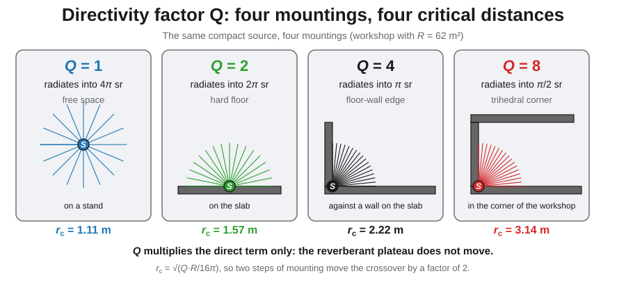
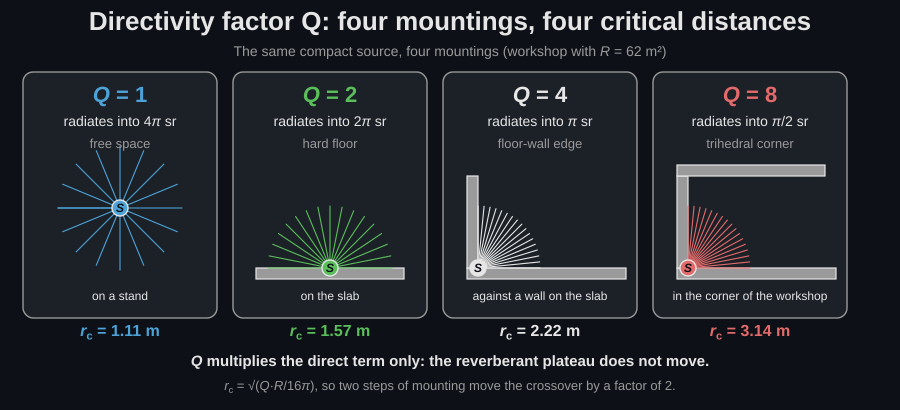
Four isometric cells in a row showing the same compact source radiating into a shaded solid angle: free space on a stand into 4 pi steradians with Q equal to 1, on the slab into 2 pi with Q equal to 2, against a wall on the slab into pi with Q equal to 4, and in a trihedral corner into pi over 2 with Q equal to 8; each cell prints the critical distance the mounting gives in a workshop with a room constant of 62 square metres, 1.11, 1.57, 2.22 and 3.14 metres

The four values of $Q$ as four mountings, with the critical distance each produces in the 12 × 8 × 4 m workshop of the figure below ( $R$ = 62 m²). $Q$ multiplies the direct term only: the reverberant plateau does not move, so mounting a machine in the corner raises the level near it without changing the level at the far end of the room.

from phonometry import room

field = room.steady_state_field(
    sound_power_level=90.0,     # Lw, dB re 1 pW
    surface_area=100.0,          # total boundary area S, m^2
    mean_absorption=0.2,         # mean Sabine absorption alpha_bar
)
print(round(field.room_constant, 1))          # 25.0 m^2
print(round(field.critical_distance, 2))       # 0.71 m
field.plot()                                    # direct / reverberant / total vs distance

On a room worth drawing — a 12 × 8 × 4 m workshop, $S$ = 352 m², $\overset{α}{ˉ}$ = 0.15, so $R$ = 62 m² — SteadyFieldResult.plot() draws the direct, reverberant and total levels against distance with the critical distance marked: the total curve follows the $1/ r^{2}$ direct field near the source and flattens onto the reverberant plateau beyond $r_{c}$ = 1.11 m.

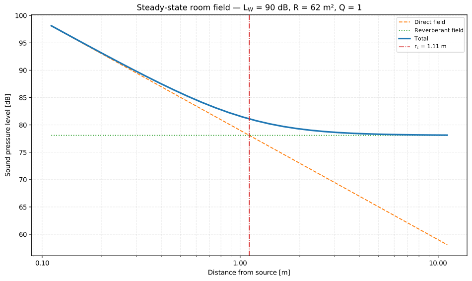
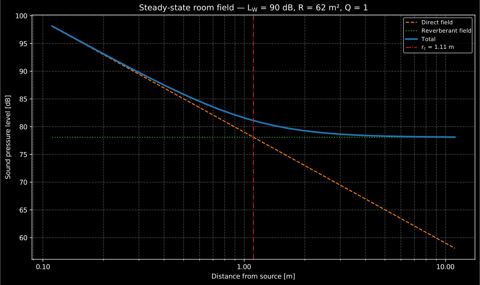
A 90 dB re 1 pW source in a 12 x 8 x 4 m workshop with a mean absorption of 0.15: within $r_{c} = 1.11$ m moving away drops the level 6 dB per doubling; beyond it the reverberant plateau takes over and only absorption, not distance, lowers the level (Bies 5e, §6.4).

Show the code for this figure

import matplotlib.pyplot as plt
import numpy as np
from phonometry import room

field = room.steady_state_field(
    sound_power_level=90.0,     # Lw, dB re 1 pW
    surface_area=352.0,          # a 12 x 8 x 4 m workshop
    mean_absorption=0.15,
)

# One line: direct, reverberant and total levels with rc marked.
field.plot()
plt.show()

# By hand, from the result's fields:
fig, ax = plt.subplots()
ax.semilogx(field.distances, field.direct, "--", label="Direct field")
ax.semilogx(field.distances, field.reverberant, ":", label="Reverberant field")
ax.semilogx(field.distances, field.total, label="Total")
ax.axvline(field.critical_distance, ls="-.",
           label=f"rc = {field.critical_distance:.2f} m")
ax.set_xlabel("Distance from source [m]")
ax.set_ylabel("Sound pressure level [dB]")
ax.legend()
plt.show()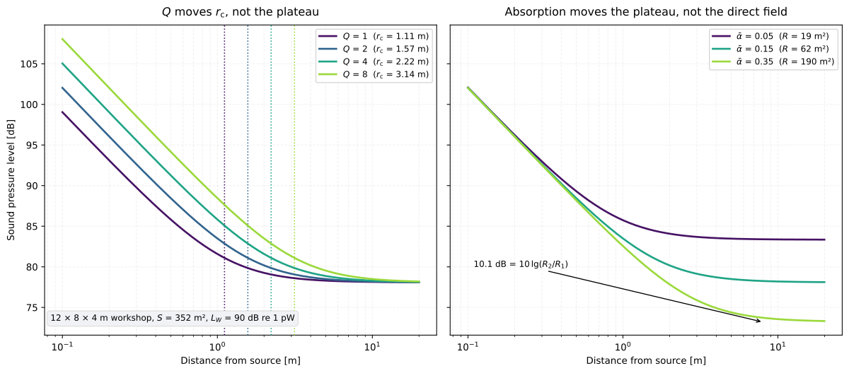

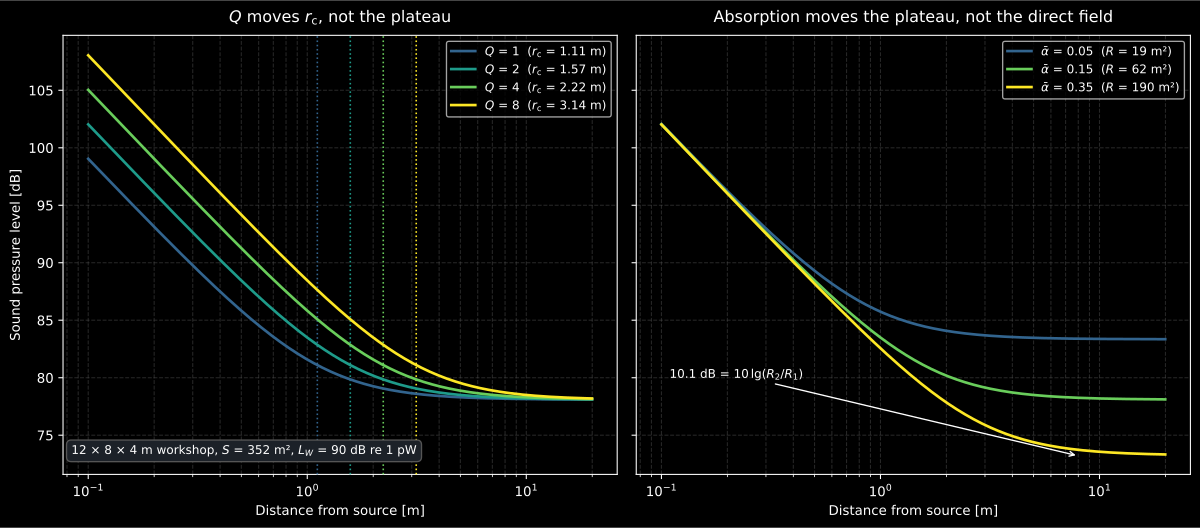
Left: $Q$ moves the crossover, not the plateau. Doubling $Q$ raises the direct field by 3 dB and pushes $r_{c}$ out by $2$ , but the reverberant level far from the source is identical in all four curves, because $Q$ never enters the $4/ R$ term. Right: absorption does the opposite. Stepping $\overset{α}{ˉ}$ from 0.05 to 0.35 takes the room constant from 18.5 m² to 189.5 m² and the plateau from 83.3 dB to 73.2 dB — 10.1 dB, exactly $10 l g (R_{2} / R_{1})$ — while the near-field asymptote does not move. That is the precise content of “beyond $r_{c}$ only absorption, not distance, lowers the level”, and it is a seven-fold increase in absorption for 10 dB.

Show the code for this figure

import matplotlib.pyplot as plt
import numpy as np
# `room` is the import of the steady-state block above.

grid = np.logspace(-1, 1.3, 200)
fig, (left, right) = plt.subplots(1, 2, figsize=(12.5, 5.0), sharey=True)
for q in (1.0, 2.0, 4.0, 8.0):
    field = room.steady_state_field(sound_power_level=90.0, surface_area=352.0,
                                    mean_absorption=0.15, distances=grid,
                                    directivity=q)
    left.semilogx(field.distances, field.total, label=f"Q = {q:g}")
    left.axvline(field.critical_distance, ls=":", alpha=0.5)
for absorption in (0.05, 0.15, 0.35):
    field = room.steady_state_field(sound_power_level=90.0, surface_area=352.0,
                                    mean_absorption=absorption, distances=grid,
                                    directivity=2.0)
    right.semilogx(field.distances, field.total,
                   label=rf"$\bar\alpha$ = {absorption:g}")
for ax in (left, right):
    ax.set_xlabel("Distance from source [m]")
    ax.legend()
left.set_ylabel("Sound pressure level [dB]")
plt.show()

The building blocks are exposed individually, so an emission measurement can flow straight into a level prediction:

from phonometry import room

R = room.room_constant(100.0, 0.2)                     # Bies room constant, 25 m^2
print(round(float(room.critical_distance(R)), 3))      # 0.705 m (Q = 1)
print(round(float(room.steady_state_spl(90.0, 5.0, R)), 2))   # level at 5 m, dB

$Q$ enters twice, and the second time is a modelling choice. It always concentrates the direct field into $Q / (4 π r^{2})$ . Whether it also raises the radiated power depends on the source’s own impedance behaviour (Norton & Karczub 2e, Table 4.5), and steady_state_spl exposes that as source_model. A constant-power source radiates $Π_{0}$ wherever it stands — the default, and the right model for a machine whose output is set by its internal losses. A constant-volume source is loaded by the reflecting boundaries and radiates $Π_{0} Q$ , so a corner adds $10 l g Q$ = 9 dB on top of the directivity concentration; that is the conservative upper bound to quote when the source type is unknown. A constant-pressure source radiates $Π_{0} / Q$ , the theoretical lower bound.

# `room` and `R` come from the block above.
print([round(float(room.steady_state_spl(90.0, 5.0, R, directivity=8.0,
                                         source_model=model)), 1)
       for model in room.SOURCE_POWER_MODELS])
# [82.7, 91.7, 73.7] dB for constant_power / constant_volume / constant_pressure

Eighteen decibels between the bounds, for one corner-mounted machine. The standards leave the choice to the engineer, so state which model a predicted level assumes in any report that carries it.

What the reverberant plateau is worth. Because the plateau is $L_{W} + 10 l g (4/ R)$ , adding absorption changes it by $10 l g (R_{2} / R_{1})$ : doubling the room constant buys 3 dB, and a realistic retrofit in a hard workshop buys perhaps 5 to 8 dB before the $(1 - \overset{α}{ˉ})$ denominator saturates the return. Two consequences follow. Treating the room only helps receivers beyond the critical distance, so an operator standing at the machine gains nothing from an acoustic ceiling and the fix there is the source, an enclosure or a screen. And the flat plateau is an idealisation: in a large or flat industrial space the level keeps falling with distance well past the predicted crossover, so this model over-predicts the level far from the source, under-predicts the benefit of distance, and the crossover is best read as an order-of-magnitude landmark rather than a boundary.

Kuttruff’s reverberation distance ( $r_{c} = A /16 π$ for $Q = 1$ ) uses the Sabine absorption area $A = S \overset{α}{ˉ}$ rather than the room constant $R = A / (1 - \overset{α}{ˉ})$ ; the two coincide for a small $\overset{α}{ˉ}$ , and this module uses $R$ so that $r_{c}$ is exactly the crossover of its own steady_state_spl. Pass characteristic_impedance=rho_c to add the Bies $10 lo g_{10} (ρ c /400)$ term (about +0.14 dB at 20 °C).

Where the statistics fade. The Schroeder frequency $f_{s} = 2000 T / V$ ( $V$ in m³, $T$ in s) roughly marks the modal-to-diffuse transition, a heuristic crossover rather than a sharp cutoff: well below it discrete modes dominate and the diffuse assumptions of $R$ and $r_{c}$ grow unreliable, well above it the modes overlap and this statistical picture holds. Borderline rooms warrant a band-by-band check.

The constant 2000 is one line of reasoning away from material this page already carries. Damping gives each mode a half-power bandwidth of about $2.2/ T$ hertz, so the modes of a decaying room are overlapping resonances rather than lines; the number of them per hertz is the modal density derived in §3, which grows as the square of frequency, so overlap becomes inevitable above some frequency. Ask for roughly three modes inside one bandwidth — set $3 \approx (2.2/ T) (4 π V f^{2} / c_{0}^{3})$ — and solving for $f$ gives $f_{s} \approx 2000 T / V$ at $c_{0} \approx 343$ m/s. Three things follow. The constant encodes a choice of how much overlap counts as diffuse, so stricter authors quote 4000 for the same physics. A large room reaches the transition at a lower frequency purely because it has more modes at every frequency. And the transition is soft, so a band straddling $f_{s}$ should be checked position by position rather than trusted. The mode-ladder figure of §3 shows the crossing directly: its modal density passes one mode per hertz right around the marked Schroeder frequency.

from phonometry import room
print(round(float(room.schroeder_frequency(1.0, 200.0)), 0))   # 141 Hz

`steady_state_field()` parameters

Parameter	Type	Units	Range / default	Notes
`sound_power_level`	float	dB re 1 pW	—	Source power level `Lw`
`surface_area`	float	m²	> 0	Total boundary area `S`
`mean_absorption`	float	—	`(0, 1)`	Mean Sabine absorption `alpha_bar`
`distances`	1D array, optional	m	> 0	Distance grid (default: `0.1 rc` to `10 rc`)
`directivity`	float	—	> 0, default 1	Source directivity factor `Q`
`characteristic_impedance`	float, optional	Pa·s/m	> 0	Adds the `10 lg(rho c / 400)` term

Returns a SteadyFieldResult (distances, direct, reverberant, total, critical_distance, room_constant) with .plot(). The pieces room_constant, critical_distance, schroeder_frequency and steady_state_spl are also callable directly (each accepting per-band arrays).

3. Modes of a rectangular room

Below the Schroeder frequency the statistical picture of §2 breaks down and the room is a handful of discrete standing waves. For the rigid-walled shoebox the wave equation separates and the eigenfrequencies are exact (Long, Architectural Acoustics 2e, Eq. (8.43)):

f_{n_{x} n_{y} n_{z}} = \frac{c _{0}}{2} (\frac{n _{x}}{l _{x}})^{2} + (\frac{n _{y}}{l _{y}})^{2} + (\frac{n _{z}}{l _{z}})^{2},

with non-negative integer orders counting nodal planes on each axis. How many of the three orders are non-zero names the family: axial (one, a wave bouncing between one pair of walls, the loudest), tangential (two, grazing four walls, about 3 dB weaker) and oblique (three, involving all six, weaker still).

from phonometry import room

modes = room.room_modes(
    (7.0, 5.0, 3.0),            # lx, ly, lz in metres
    max_frequency=100.0,
    speed_of_sound=344.0,
    reverberation_time=0.8,     # optional: carries the Schroeder frequency
)
print(modes.orders[0], round(float(modes.frequencies[0]), 1))  # [1 0 0] 24.6 Hz
print(modes.count_by_kind())   # {'axial': 7, 'tangential': 10, 'oblique': 4}
print(round(modes.schroeder_frequency, 0))                     # 175 Hz
modes.plot()                    # mode ladder by family + modal density

Counting lattice points inside the positive octant of a sphere of radius $k = 2 π f / c_{0}$ , with the half- and quarter-weight corrections for the points on the coordinate planes and axes, gives the smooth integrated mode count (Eq. (8.45), after Morse and Pierce) and its derivative the modal density (Eq. (8.46)):

N (f) = \frac{4 π}{3} V (\frac{f}{c _{0}})^{3} + \frac{π}{4} S (\frac{f}{c _{0}})^{2} + \frac{L}{8} \frac{f}{c _{0}}, \frac{d N}{df} = \frac{4 π V f ^{2}}{c _{0}^{3}} + \frac{π S f}{2 c _{0}^{2}} + \frac{L}{8 c _{0}},

with the volume $V$ , the total wall area $S$ and the sum $L$ of the twelve edge lengths. These are asymptotic estimates: below a few dozen modes the exact enumeration of room_modes is the honest answer, while high up they are accurate and much cheaper.

from phonometry import room

room_dims = (7.0, 5.0, 3.0)
print(round(float(room.room_mode_count(200.0, room_dims, speed_of_sound=344.0)), 1))
# 128.5, against 128 modes actually enumerated below 200 Hz
print(round(float(room.room_modal_density(1000.0, room_dims, speed_of_sound=344.0)), 1))
# 34.3 modes/Hz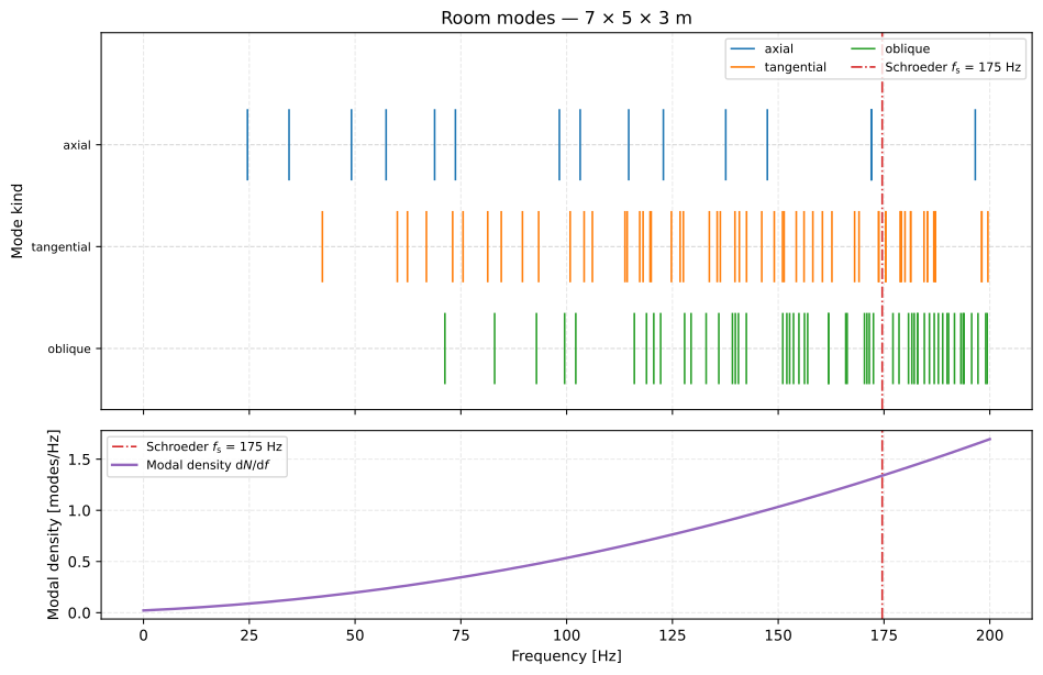

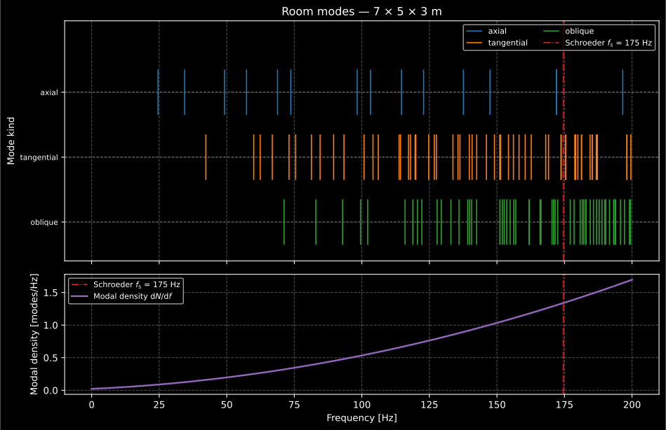
Mode ladder of a 7 by 5 by 3 metre room up to 200 Hz, one raster row per family (axial, tangential, oblique) and the modal density curve below, both marked with the 175 Hz Schroeder frequency

The 7 x 5 x 3 m room of Long’s Table 8.1 up to 200 Hz. Below about 60 Hz the axial modes stand alone and each is separately audible; by the 175 Hz Schroeder frequency ( $T = 0.8$ s) the oblique family has filled in and the modal density has passed one mode per hertz, which is where the statistical field of §2 takes over.

Show the code for this figure

import matplotlib.pyplot as plt
import numpy as np
# `room` is the import of the room_modes block above.

# Long, Architectural Acoustics 2nd ed., Table 8.1.
modes = room.room_modes((7.0, 5.0, 3.0), max_frequency=200.0,
                        speed_of_sound=344.0, reverberation_time=0.8)

# One line: the mode ladder by family with the modal density below.
modes.plot()
plt.show()

# By hand: scatter the eigenfrequencies, one row per family.
kinds = np.asarray(modes.kinds)
rows = {"axial": 0, "tangential": 1, "oblique": 2}
fig, ax = plt.subplots()
for name, y in rows.items():
    sel = kinds == name
    ax.vlines(np.asarray(modes.frequencies)[sel], y, y + 0.8, label=name)
ax.axvline(modes.schroeder_frequency, ls=":", color="k",
           label=f"Schroeder {modes.schroeder_frequency:.0f} Hz")
ax.set_yticks([0.4, 1.4, 2.4], list(rows))
ax.set_xlabel("Frequency [Hz]")
ax.legend()
plt.show()

`room_modes()` parameters

Parameter	Type	Units	Range / default	Notes
`dimensions`	3-tuple	m	> 0	Room dimensions `(lx, ly, lz)`
`max_frequency`	float	Hz	> 0, default 200	Highest mode enumerated
`speed_of_sound`	float	m/s	> 0, default 343	`c0`
`reverberation_time`	float, optional	s	> 0	Adds the Schroeder frequency to the result

Returns a RoomModesResult (orders, frequencies, kinds, dimensions, speed_of_sound, schroeder_frequency, plus the volume, surface_area and edge_length properties and count_by_kind()) with .plot(). The pieces room_mode_frequency, room_mode_count and room_modal_density are callable directly.

Reading the ladder. Two things matter more than any single frequency. Modes that coincide colour the sound: if the dimensions are low integer multiples of one another the energy coalesces into a few frequencies, which is why a cubic room is the worst possible listening room and why the ratio tables of Bolt and others exist. And modes crowd together as frequency rises, until they merge into the continuum the statistical model of §2 assumes.

Degeneracy is a countable thing, not a matter of taste. Three rooms of the same 105 m³ volume, enumerated up to 200 Hz, hold about the same number of modes and a completely different number of frequencies.

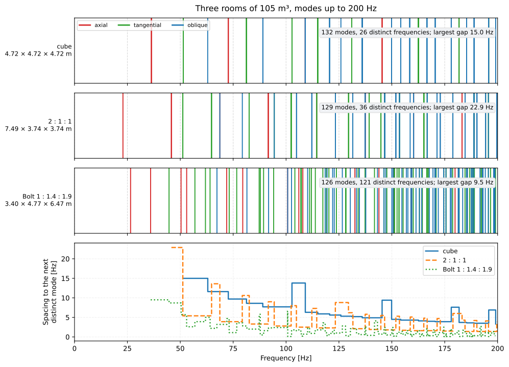
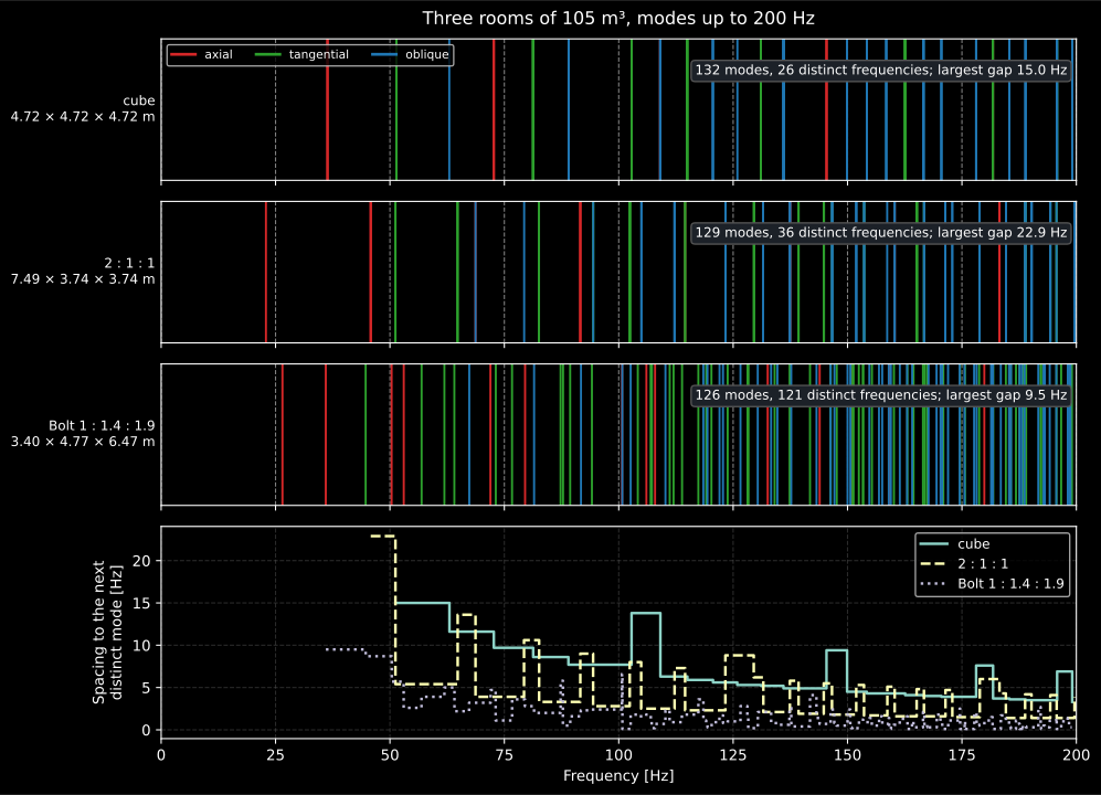
Three stacked raster rows of mode ticks up to 200 hertz for three rooms of the same 105 cubic metre volume, coloured by family: a 4.72 metre cube whose ticks pile onto a few frequencies separated by wide empty gaps, a 7.49 by 3.74 by 3.74 metre room slightly better, and a Bolt-ratio room of 3.40 by 4.77 by 6.47 metres whose ticks are strewn almost evenly; a fourth panel below plots the spacing between consecutive distinct frequencies for the three rooms

The same volume in three shapes. The 4.72 m cube enumerates 132 modes at only 26 distinct frequencies — a five-fold pile-up — with a 15.0 Hz hole in the ladder; the 2:1:1 room manages 36 distinct frequencies out of 129 and an even wider 22.9 Hz hole; the Bolt-ratio room 1 : 1.4 : 1.9 gives 121 distinct frequencies out of 126 and its largest gap is 9.5 Hz. Piled-up frequencies are heard as coloration on those notes, and the gaps between them as notes the room swallows. This is what proportion buys, and it costs nothing at design time.

Show the code for this figure

import matplotlib.pyplot as plt
import numpy as np
# `room` is the import of the mode block above.

volume = 105.0
half = (volume / 2.0) ** (1 / 3)
bolt = (volume / (1.0 * 1.4 * 1.9)) ** (1 / 3)
shapes = {
    "cube": (volume ** (1 / 3),) * 3,
    "2 : 1 : 1": (2 * half, half, half),
    "Bolt 1 : 1.4 : 1.9": (bolt, 1.4 * bolt, 1.9 * bolt),
}
fig, axes = plt.subplots(len(shapes), 1, sharex=True)
for ax, (name, dims) in zip(axes, shapes.items()):
    modes = room.room_modes(dims, max_frequency=200.0)
    freqs = np.asarray(modes.frequencies)
    ax.vlines(freqs, 0, 1)
    ax.set_ylabel(f"{name}\n{np.unique(np.round(freqs, 1)).size} distinct")
axes[-1].set_xlabel("Frequency [Hz]")
plt.show()

Where the pressure is. The mode shape of $(n_{x}, n_{y}, n_{z})$ in a rigid box is the product of cosines $cos (n_{x} π x / l_{x}) cos (n_{y} π y / l_{y}) cos (n_{z} π z / l_{z})$ , and two consequences of that one formula are worth more than the whole frequency list. Every mode has a pressure antinode at every corner, because every cosine is at $\pm 1$ there — which is why a subwoofer and a bass trap both belong in a corner, and why a microphone in one over-reads the low bands. And an axis whose order is odd has a node at its midpoint, so a listening position at exactly half a room dimension sits in a null of every odd axial mode on that axis; low-frequency measurement positions are kept off the mid-planes for the same reason. The source matters as much as the receiver: a source sitting on a mode’s nodal plane cannot drive that mode at all. What the rigid-wall model cannot tell you is how strongly each resonance rings, since that is set by the damping it omits — for that, mesh the room and run the 2D FDTD solver.

Validation

The implementations are checked against the closed forms and the source texts’ own numeric anchors (see the conformance report):

the direct-sound amplitude $1/ (4 π r)$ and delay $r / c$ (exact geometry), the audible image count (Kuttruff 6e, Eq. (9.23)) and the reflection density (Eq. (4.6));
the Eyring reverberation time recovered from the decay of the synthetic RIR in the near-cubic limit (documented ≈ 10 % tolerance), and an independent 2D FDTD solver reproducing the rigid-wall echo delay and the uniform-damping $T_{60}$ ;
the room constant, the critical distance as the exact direct/reverberant crossover, the Schroeder frequency (Kuttruff’s classroom example, $V = 200$ m³, $T = 1$ s → 141 Hz) and the steady-state level (Bies 5e, Eq. (6.43));
the six modes Long prints for his 7 x 5 x 3 m room (Table 8.1: 24.6, 34.5, 42.4, 49.2, 57.4 and 60.1 Hz, reproduced within one unit of the last printed digit at his $c_{0} = 344$ m/s) and the 34 modes per hertz he states for the same room at 1 kHz (Eq. (8.46)), plus the mode count matched against the exact enumeration and the degeneracy of a cubic room.

What this guide covers

Covered
Kuttruff’s Room Acoustics (the image-source construction of §4.1, the Eyring reverberation formula used for the near-cubic check and the Schroeder frequency of §3.6), Vorländer’s Auralization (the mirror-source model of Chapter 11, its reflection-factor and delay expressions) and Allen & Berkley’s reflection-order decomposition, all implemented by room.image_source_rir; and the Bies, Hansen & Howard steady-state room field of §6.4 (room constant, directivity $Q$ , critical distance) implemented by room.steady_state_field, room.room_constant, room.critical_distance, room.steady_state_spl and room.schroeder_frequency; and Long’s Architectural Acoustics Chapter 8 (the rectangular-room eigenfrequencies of Eq. (8.43) with their axial/tangential/oblique classification, and the Morse/Pierce mode count and modal density of Eqs. (8.45) and (8.46)) implemented by room.room_modes, room.room_mode_frequency, room.room_mode_count and room.room_modal_density.
Not covered
The image-source model captures specular reflections only: no diffraction and no diffuse scattering, so an elongated room’s true decay runs slower than the diffuse-field Eyring estimate it is checked against (the anisotropy the Fitzroy and Arau-Puchades models of the reverberation-prediction guide were built to correct). Kuttruff’s alternative reverberation distance (using the Sabine absorption area in place of the room constant) is cited for comparison but not implemented: steady_state_field and critical_distance always use the Bies room-constant formulation. The mode calculator assumes rigid walls and a rectangular plan: it gives the eigenfrequencies, not the pressure amplitude at a listening position, and it says nothing about damping, mode shape or a non-shoebox geometry. For those, mesh the room and run the 2D FDTD solver. Bolt’s preferred dimension ratios are discussed but not tabulated.

References

Allen, J. B., & Berkley, D. A. (1979). Image method for efficiently simulating small-room acoustics. The Journal of the Acoustical Society of America, 65(4), 943-950. https://doi.org/10.1121/1.382599The reflection-count decomposition of the rectangular-room image lattice used in §1.
Bies, D. A., Hansen, C. H., & Howard, C. Q. (2017). Engineering noise control (5th ed.). CRC Press. https://doi.org/10.1201/9781351228152The steady-state room field and the room constant of §2 (§6.4).
Kuttruff, H. (2016). Room acoustics (6th ed.). CRC Press. https://doi.org/10.1201/9781315372150The image-source construction (§4.1), the Eyring reverberation and reverberation distance (§5.5–5.6) and the Schroeder frequency (§3.6) of this page.
Long, M. (2014). Architectural acoustics (2nd ed.). Academic Press. https://doi.org/10.1016/C2012-0-03257-5The rectangular-room modes of §3: the eigenfrequencies of Equation (8.43), the Table 8.1 example room and the Morse/Pierce mode count and modal density of Equations (8.45) and (8.46).
Vorländer, M. (2020). Auralization: Fundamentals of acoustics, modelling, simulation, algorithms and acoustic virtual reality (2nd ed.). Springer. https://doi.org/10.1007/978-3-030-51202-6The mirror-source model of §1 (Chapter 11), with the reflection-factor and delay expressions.

Created and maintained by José Manuel Requena Plens ORCID All projects

Image Sources and the Steady-State Room Field

1. Image-source room impulse response

image_source_rir() parameters

Choosing max_order, duration and fs

2. Steady-state room field

steady_state_field() parameters

3. Modes of a rectangular room

room_modes() parameters

Validation

What this guide covers

See also

References

`image_source_rir()` parameters

Choosing `max_order`, `duration` and `fs`

`steady_state_field()` parameters

`room_modes()` parameters