Underwater sound propagation
Standards: ISO 18405Key references: Francois & Garrison 1982Ainslie & McColm 1998Thorp 1967Chen & Millero 1977Wong & Zhu 1995Del Grosso 1974Mackenzie 1981Leroy & Parthiot 1998+7 more
This page computes what the sea does to a sound level in closed form, without simulating a field. By the end you can put a number on the propagation loss of a path, choose the absorption and sound-speed models that suit your water, follow Weston’s four shallow-water regimes as the sea floor takes over from geometry, balance a passive or active sonar equation and invert it for a detection range, evaluate the seabed reflection loss that sets those regimes, and build an ambient-noise spectrum from wind, thermal and ship-traffic terms. The reference levels every result is expressed in are on the Underwater acoustics page; when refraction and boundaries decide the answer, the solvers take over.
Propagation loss
Section titled “Propagation loss”Two quantities, and ISO 18405 keeps them apart. Propagation loss is the difference between the source level in a specified direction and the mean-square sound pressure level at a specified position, , referred to 1 m² (clause 3.4.1.4). Transmission loss is the reduction in a specified level between two specified points (clause 3.4.1.3). The sonar equation needs the source-referred quantity, so what this page computes is a propagation loss, and that is what the function is called. The standard deprecates each name as a synonym of the other, in both directions, which is why so much of the literature calls this quantity a transmission loss and why this library stopped. Either quantity has to be quoted with the averaging time and the frequency range it applies to. Weston’s regimes below are the same quantity on the same axis.
The propagation loss is
Geometrical spreading is (spherical), (cylindrical) or
spherical up to a transition range and cylindrical beyond it ("practical"). The
volume absorption (dB/km) comes
from Francois-Garrison (model="francois-garrison", 1982, the default and
the reference), Ainslie-McColm ("ainslie-mccolm", 1998) or Thorp
("thorp", 1967, frequency-only); the first two agree to within ~10 % across
100 Hz-1 MHz.
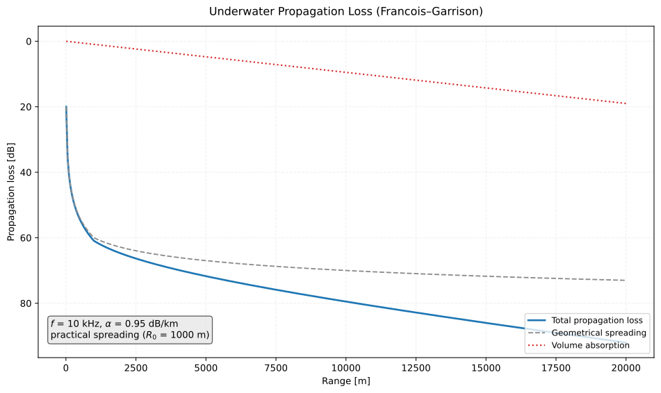
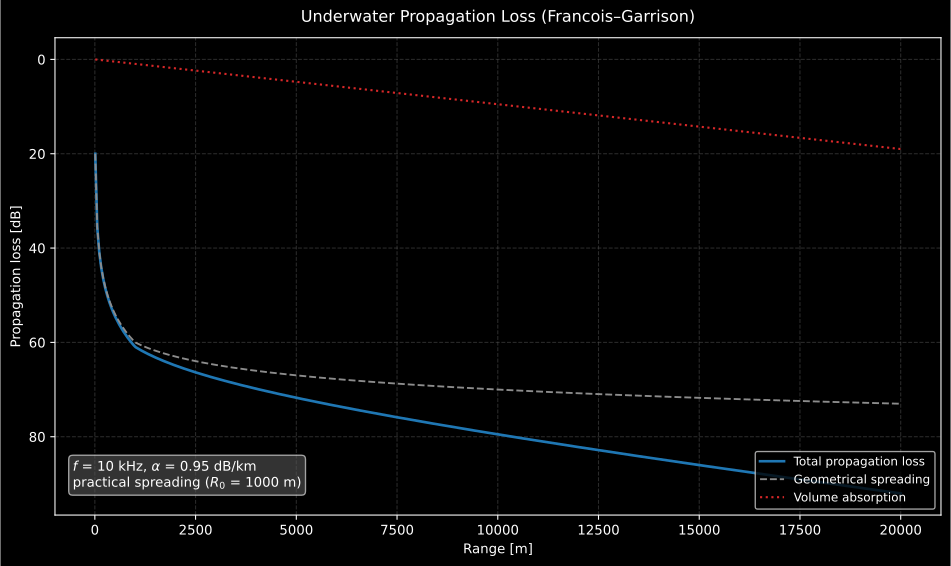
The two terms trade places with range, which is why they are drawn apart. Out to the 1 km transition the loss is spreading and almost nothing else: 61.0 dB total against 60.1 dB of spreading. Past it the spreading law halves to and the term takes over the growth: at 20 km, 92.0 dB total is 73.0 dB of spreading plus 19.0 dB of absorption at 0.95 dB/km. At 10 kHz absorption never overtakes spreading over this range; at 100 kHz it would have done so inside the first kilometre.
Show the code for this figure
import matplotlib.pyplot as pltimport numpy as npfrom phonometry import underwater
# 10 kHz at 10 °C, 35 ppt, 100 m depth; practical spreading with R0 = 1000 m.ranges = np.linspace(10.0, 20_000.0, 400)pl = underwater.propagation_loss(ranges, 10e3, law="practical",                                  transition_range=1000.0, temperature_c=10.0,                                  salinity=35.0, depth=100.0)print(f"alpha = {pl.absorption_coefficient:.2f} dB/km")   # alpha = 0.95 dB/kmpl.plot()   # total PL with the spreading and absorption contributionsplt.show()
import numpy as npfrom phonometry import underwater
ranges = np.linspace(10.0, 20_000.0, 400)pl = underwater.propagation_loss(ranges, 10e3, law="practical", transition_range=1000.0, temperature_c=10.0, salinity=35.0, depth=100.0)print(round(pl.absorption_coefficient, 3), round(float(pl.pl[-1]), 1))# 0.95 dB/km, 92.0 dB at 20 km
# The same case on the other two absorption models, so the agreement claim# above is checkable rather than asserted:for model in ("ainslie-mccolm", "thorp"): other = underwater.propagation_loss(ranges, 10e3, law="practical", transition_range=1000.0, temperature_c=10.0, salinity=35.0, depth=100.0, model=model) print(model, round(other.absorption_coefficient, 3)) # 0.973 / 1.15
pl.plot() # PL vs range with the spreading/absorption split (needs matplotlib)Two arguments in that call decide more than they look. depth is only the depth
at which the absorption coefficient is evaluated (a representative depth along
the path, because falls with pressure) and it is not the water
depth and does not set the spreading law. is the range at which the
wavefront has filled the duct, so it is of the order of the water depth in a
shallow waveguide, or of the channel thickness in a SOFAR duct: a 100 m channel
takes near 100 m, not the 1 km used above, which belongs to a deep-water
path. The choice is not cosmetic. Against the figure of merit of 87 dB worked
below, spherical-only spreading puts detection at 8.7 km and the practical law
with m at 15.8 km. The same ocean, seven kilometres apart.
The absorption model matters less, and it is worth seeing how much less.
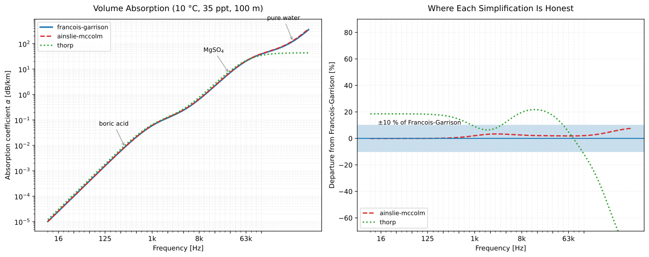
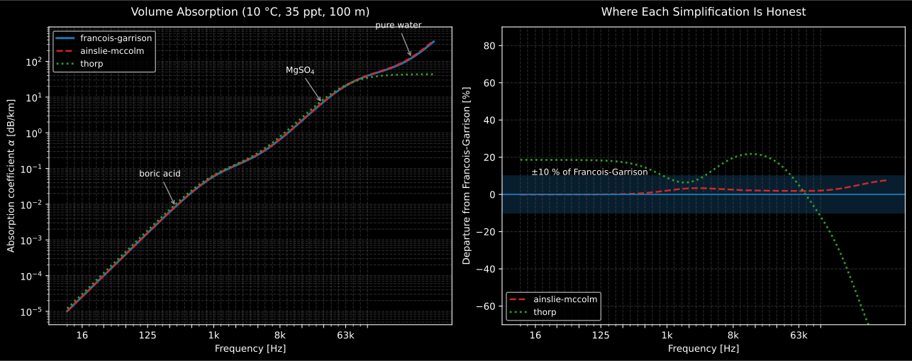
Ainslie-McColm stays inside ±10 % of the Francois-Garrison reference across the whole band, which is what makes it a legitimate substitute. Thorp does not: it runs about 20 % high below a few hundred hertz and collapses above ~60 kHz, because it is a frequency-only fit with 4 °C water near 1000 m baked into it and no temperature, salinity or depth to give.
Show the code for this figure
import matplotlib.pyplot as pltimport numpy as np
freqs = np.logspace(1.0, 6.0, 500)env = {"temperature_c": 10.0, "salinity": 35.0, "depth": 100.0}alpha = {m: np.asarray(underwater.seawater_absorption(freqs, model=m, **env))         for m in ("francois-garrison", "ainslie-mccolm", "thorp")}
fig, (ax_a, ax_r) = plt.subplots(1, 2, figsize=(13.5, 5.4))for name, style in (("francois-garrison", "-"), ("ainslie-mccolm", "--"),                    ("thorp", ":")):    ax_a.loglog(freqs, alpha[name], style, label=name)    if name != "francois-garrison":        ax_r.semilogx(freqs, 100.0 * (alpha[name] / alpha["francois-garrison"] - 1.0),                      style, label=name)ax_a.set(xlabel="Frequency [Hz]", ylabel="alpha [dB/km]")ax_r.set(xlabel="Frequency [Hz]", ylabel="Departure from Francois-Garrison [%]",         ylim=(-70, 90))for ax in (ax_a, ax_r):    ax.grid(True, which="both", alpha=0.3)    ax.legend()plt.show()
Weston’s shallow-water regimes
Section titled “Weston’s shallow-water regimes”Fixing the spreading law by hand works offshore, but in shallow water the law changes with range as the sea floor takes over. Weston’s energy-flux theory, as set out in Ainslie §9.1.1.2, derives the four successive regimes and the ranges at which they hand over, from the seabed reflectivity alone:
| Regime | Propagation factor | Loss law | Ends at |
|---|---|---|---|
| Spherical | |||
| Cylindrical | |||
| Mode stripping | |||
| Single mode | Eq. (9.54), exponential | steeper than | — |
Here is the range, the water depth, the acoustic wavenumber in the water column, the critical grazing angle set by the water and sediment sound speeds, the reflection loss gradient in nepers per radian () and the Weston effective depth: the level a short distance below the true seabed at which a pressure-release boundary appears to lie, so and the two letters are not interchangeable (which is the whole of the errata note below).
weston_propagation_loss assembles the composite loss and returns each regime’s
own law alongside it; the boundaries field carries the three transition ranges
plus the waveguide cut-off frequency and the number of cut-on modes. What it
returns is a propagation loss : the incoherent,
range-averaged ratio of the received to the source mean-square pressure, with
the absorption term added separately. For the geometries of this page it is
directly comparable with the propagation loss above and with the depth-averaged
modal result. The difference between the two ISO 18405 quantities is the
reference-range convention, not the physics, which is why the two are plotted
on the same axis.
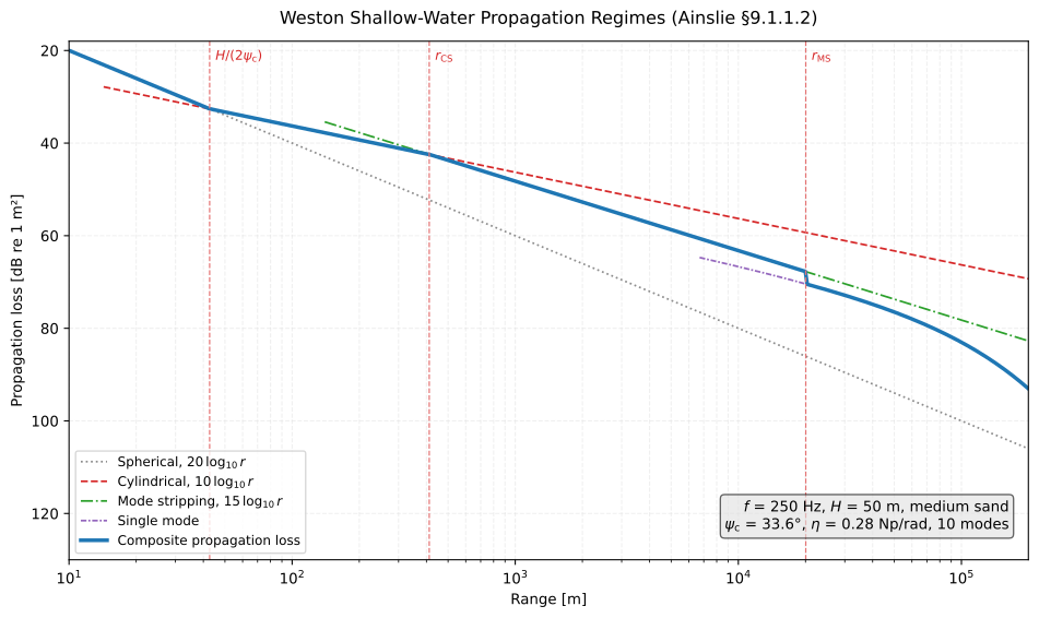
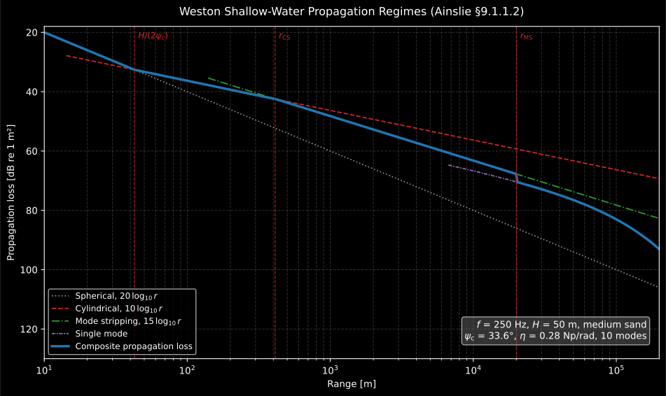
Nothing here was chosen: the three hand-overs at 42.7 m, 411.8 m and 20.1 km come out of the seabed alone, through the 33.6° critical angle and the 0.278 Np/rad reflection-loss gradient of medium sand in 50 m of water. The composite is the lower envelope of the four dashed laws, so the loss steepens in stages: 32.6 dB at the first boundary, 42.4 dB at the second, 67.7 dB at the third. Sand is the reason the middle two regimes exist at all: a harder seabed pushes the hand-overs out and a softer one strips the modes sooner.
Show the code for this figure
import matplotlib.pyplot as pltimport numpy as npfrom phonometry import underwater
# 50 m of water over medium sand (Ainslie Table 9.1) at 250 Hz.ranges = np.logspace(1.0, 5.3, 500)res = underwater.weston_propagation_loss(ranges, 250.0, 50.0, seabed="sand",                                         source_depth=10.0, receiver_depth=25.0)b = res.boundariesprint(f"psi_c = {np.degrees(b.critical_angle_rad):.1f} deg, eta = {b.reflection_loss_gradient_np_per_rad:.2f} Np/rad")res.plot()   # composite loss with each regime law and the boundariesplt.show()
from phonometry import underwater
b = underwater.weston_regime_boundaries(250.0, 50.0, seabed="sand")print(b.cylindrical_to_mode_stripping) # r_CS, in metresprint(b.cutoff_frequency, b.mode_count) # ducted propagation needs f > f_cprint(underwater.reflection_loss_gradient("sand")) # 0.278 Np/radBecause the flux result is incoherent it describes the range-averaged field, which is exactly what makes it a reference for the numerical solvers of Underwater propagation solvers. Set the critical angle to 90° and the loss gradient to zero and the cylindrical branch reduces to , the exact many-mode limit of an ideal waveguide; the depth- and range-averaged normal-mode loss lands on it to within a decibel.
Speed of sound in sea water
Section titled “Speed of sound in sea water”sea_water_sound_speed(T, S, depth, model=…) uses the UNESCO / Chen-Millero
equation (model="unesco", the default, in the Wong & Zhu 1995 ITS-90 form),
Del Grosso ("del_grosso", note the underscore, unlike the hyphenated
absorption models above), Mackenzie ("mackenzie") or Medwin
("medwin"), all 1974-1981. Depth is converted to pressure with
Leroy & Parthiot (1998). Inside the domain all four share they agree to about
1 m/s: 0.98 m/s at 25 °C, 35 ppt and 1000 m, and 0.52 m/s over the whole
upper kilometre of the profile drawn below. The choice is about validity
range, not accuracy. Mackenzie’s canonical check value is 1550.744 m/s at 25 °C,
35 ppt, 1000 m. Medwin’s six-term form is the coarsest of the family and the one
behind the classic rules of thumb
m/s per °C and
m/s per metre; it is fitted to about
1000 m in shallow, warm water, and pushed to 5000 m it leaves the others by
nearly 6 m/s, which is the one large disagreement in the family and is entirely
a matter of using it out of domain.
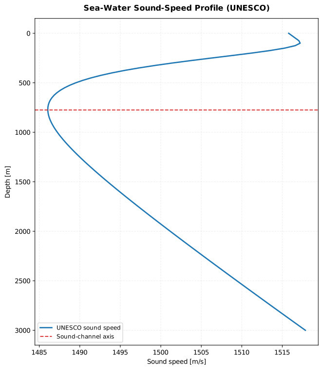
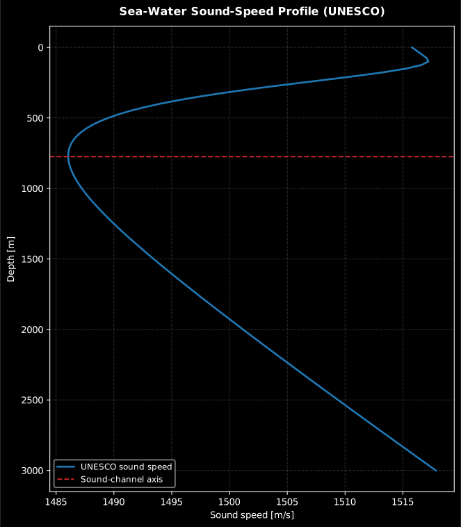
Temperature wins above the axis and pressure below it, and the turning point is the sound channel. On this profile the speed falls from 1515.79 m/s at the surface to a minimum of 1486.05 m/s at 775 m (where the water has already reached its deep temperature) and then climbs back to 1517.85 m/s at 3000 m on pressure alone, in isothermal water. The whole excursion is 32 m/s, about 2 %, which is why refraction and not absorption decides where sound goes in the deep ocean.
Show the code for this figure
import matplotlib.pyplot as pltimport numpy as npfrom phonometry import underwater
# A warm mixed layer, a thermocline down to 4 °C and an isothermal deep layer.depths = np.linspace(0.0, 3000.0, 121)temps = 4.0 + 14.0 / (1.0 + (np.maximum(depths - 80.0, 0.0) / 250.0) ** 2)profile = underwater.sound_speed_profile(depths, temps, 35.0, model="unesco")profile.plot()   # sound speed vs depth, minimum at the sound-channel axisplt.show()
import numpy as npfrom phonometry import fluids, underwater
c = fluids.sea_water_sound_speed(25.0, 35.0, 1000.0, model="mackenzie") # 1550.744depths = np.linspace(0.0, 3000.0, 121)temps = 4.0 + 14.0 / (1.0 + (np.maximum(depths - 80.0, 0.0) / 250.0) ** 2)profile = underwater.sound_speed_profile(depths, temps, 35.0, model="unesco")profile.plot() # sound speed vs depth (needs matplotlib)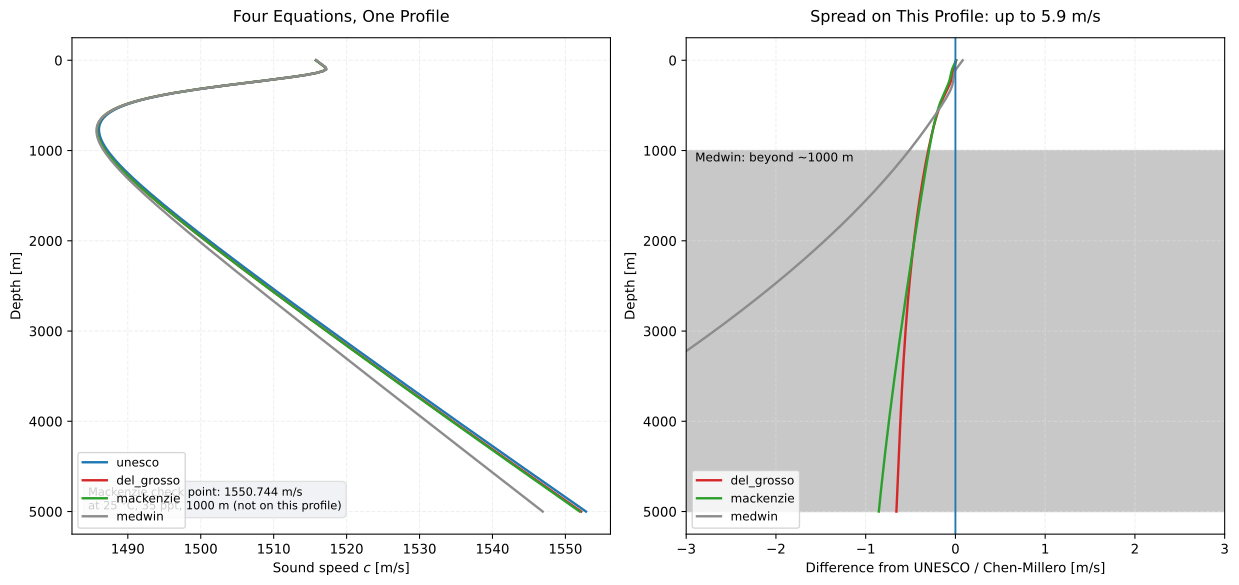
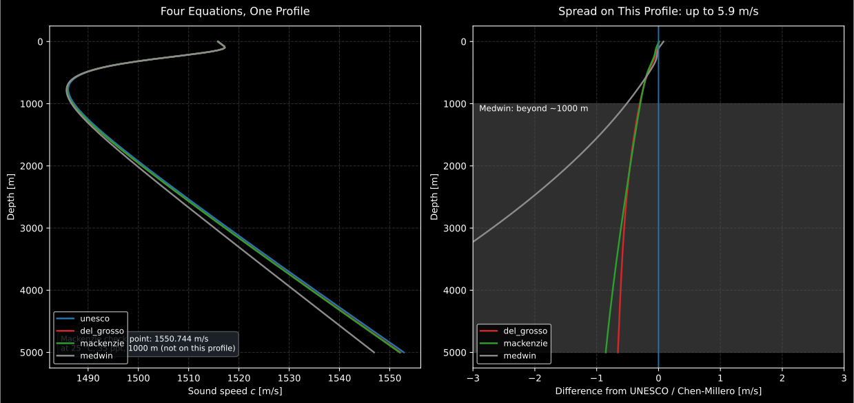
At the scale of the profile the four equations are one curve. The difference panel is the useful one: Del Grosso and Mackenzie stay within 0.85 m/s of UNESCO over the whole column, and all four are within 0.52 m/s down to 1000 m. The one large departure is Medwin below its own validity limit, which is a domain error rather than a disagreement between models.
Show the code for this figure
import matplotlib.pyplot as pltimport numpy as np
depths = np.linspace(0.0, 5000.0, 251)temps = 4.0 + 14.0 / (1.0 + (np.maximum(depths - 80.0, 0.0) / 250.0) ** 2)models = ("unesco", "del_grosso", "mackenzie", "medwin")profiles = {m: np.asarray(underwater.sound_speed_profile(    depths, temps, 35.0, model=m).speed_of_sound) for m in models}
fig, (ax_c, ax_d) = plt.subplots(1, 2, figsize=(13.0, 6.2))for m in models:    ax_c.plot(profiles[m], depths, label=m)    if m != "unesco":        ax_d.plot(profiles[m] - profiles["unesco"], depths, label=m)ax_d.axhspan(1000.0, 5000.0, color="0.9", zorder=0)   # Medwin out of domainfor ax in (ax_c, ax_d):    ax.invert_yaxis()    ax.grid(True, alpha=0.3)    ax.legend()ax_c.set(xlabel="Sound speed c [m/s]", ylabel="Depth [m]")ax_d.set(xlabel="Difference from UNESCO [m/s]", ylabel="Depth [m]", xlim=(-7, 7))plt.show()
Where the numbers come from
Section titled “Where the numbers come from”Every snippet on this page hard-codes its ocean, and a survey does not. The
temperature, salinity and depth that sea_water_sound_speed and
sound_speed_profile consume come from a CTD cast taken close to the survey
in time as well as in space; an XBT with an assumed salinity is the common
substitute, and ISO 18406 Clause 8.1.3 lists the sound-speed profile among the
auxiliary data a survey records for exactly this reason. Which model suits which
sensor follows from that: Mackenzie takes depth directly, so it fits an
echo-sounder depth, while UNESCO and Del Grosso convert depth to pressure
internally through Leroy & Parthiot.
The seabed parameters are not free constants either. The seabed class of the
Weston regimes and the , of the Rayleigh reflection come from a
grab sample or a sub-bottom survey, and the classification scheme used has to be
stated with the result: Folk or similar, as the piling standard requires.
The Wenz wind term expects a wind speed with its measurement height and
averaging period recorded, not a spot reading off the bridge; and a measured
ambient spectrum only replaces the Wenz curve where it stands clear of the
recording system’s own self-noise, which for an ordinary system approaches
sea-state-zero levels near 63 Hz and 125 Hz. Finally, , and are
properties of the receiving array and the detector, not of the sea: they arrive
from the array specification and the detection statistics, and no oceanographic
measurement will produce them.
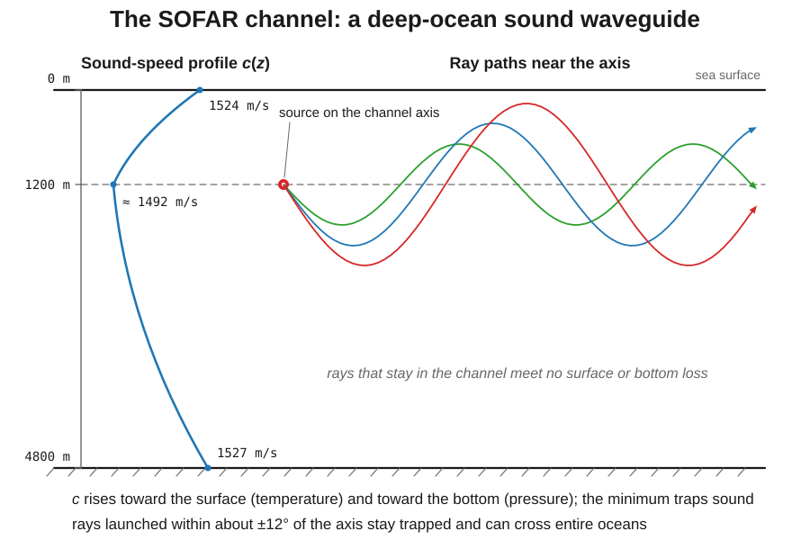
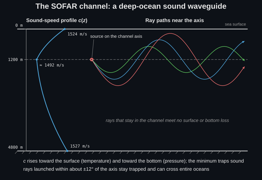
The minimum acts as a waveguide (the SOFAR channel): wavefronts that stray from the axis are refracted back toward it, while sound generated outside the channel leaks away to depth, as the simulation below shows with an intentionally exaggerated gradient. This trapping is why low-frequency sound can cross entire oceans.
Two 2D FDTD runs of a low-frequency pulse in a SOFAR-like underwater sound channel, with the c(z) profile drawn beside each field. Launched on the channel axis at 400 m depth the wavefronts keep refracting back toward the sound-speed minimum and stay trapped; launched near the surface at 150 m the energy crosses the channel and leaks away to depth. The closing seconds fade to the time-integrated energy map, showing the whole path history of each run.
Two 2D FDTD runs of a low-frequency pulse in a SOFAR-like underwater sound channel, with the c(z) profile drawn beside each field. Launched on the channel axis at 400 m depth the wavefronts keep refracting back toward the sound-speed minimum and stay trapped; launched near the surface at 150 m the energy crosses the channel and leaks away to depth. The closing seconds fade to the time-integrated energy map, showing the whole path history of each run.
At real ocean scale the channel axis sits near 1200 m, and the trapped arrivals are rays cycling about the sound-speed minimum over tens of kilometres.
Sonar equation
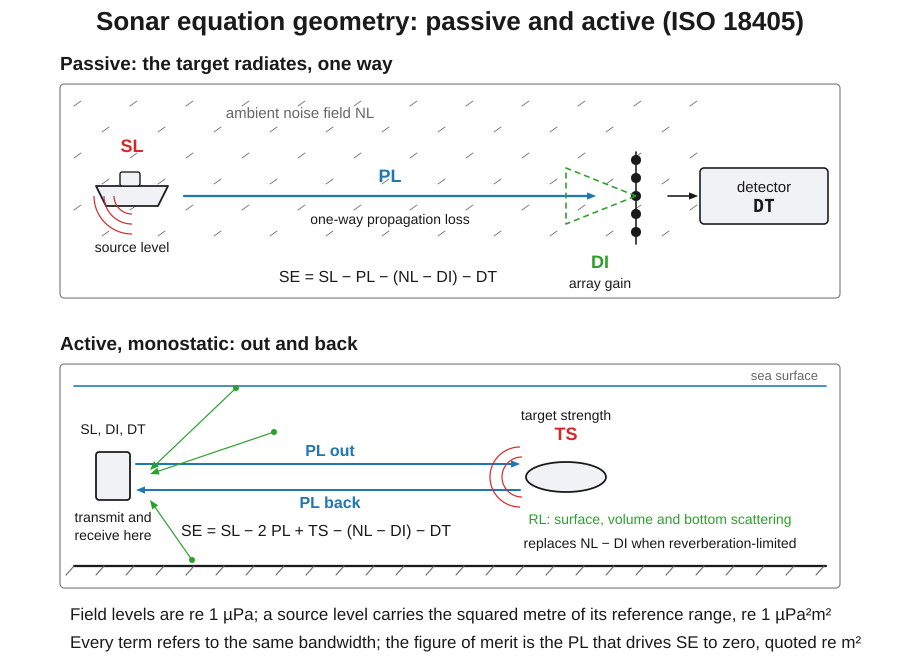
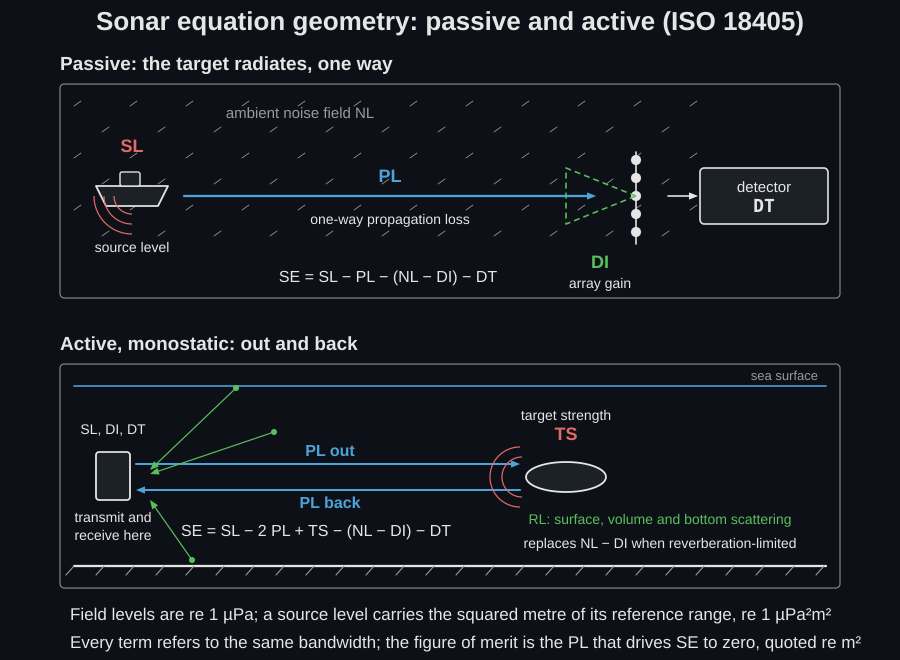
Section titled “Sonar equation”The sonar equation gives the signal excess (detection when ) and the figure of merit (the maximum allowable propagation loss at ):
or reverberation-limited with in place of .
Those two forms are two geometries. In the passive case the target radiates and the sound travels one way; in the active case the sonar radiates, the target scatters a fraction of what reaches it back, and the loss is paid twice. This is why appears doubled and appears at all. Reverberation is not ambient noise: it is the sonar’s own transmission scattered back by the surface, the volume and the seabed, so it scales with the transmitted level and replaces rather than adding to it.
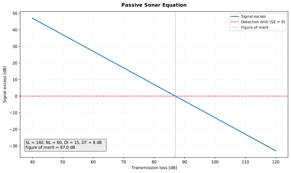
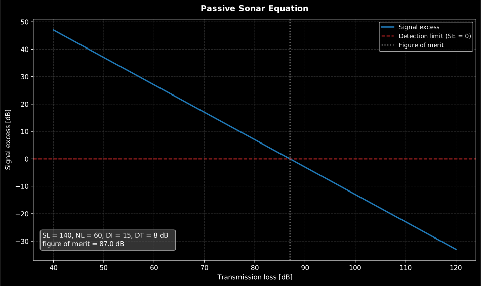
A straight line of slope −1, and its intercept is the whole design. Signal excess falls decibel for decibel with propagation loss and crosses zero at = 140 − (60 − 15) − 8 = 87.0 dB, so the sonar detects wherever the channel loses less than 87 dB and nowhere else. Every term moves the line vertically and none of them changes its slope: 6 dB more array gain buys exactly 6 dB more allowable loss, which the propagation curve then converts into a range.
Show the code for this figure
import matplotlib.pyplot as pltimport numpy as npfrom phonometry import underwater
pl = np.linspace(40.0, 120.0, 400)se = underwater.passive_sonar_equation(source_level=140.0, propagation_loss=pl,                                       noise_level=60.0, directivity_index=15.0,                                       detection_threshold=8.0)print(f"figure of merit = {se.figure_of_merit:.1f} dB")  # figure of merit = 87.0 dBse.plot()   # signal excess vs propagation loss, zero crossing at the FOMplt.show()
import numpy as npfrom phonometry import underwater
pl = np.linspace(40.0, 120.0, 400)se = underwater.passive_sonar_equation(source_level=140.0, propagation_loss=pl, noise_level=60.0, directivity_index=15.0, detection_threshold=8.0)print(se.figure_of_merit)se.plot() # signal excess vs propagation loss (needs matplotlib)The terms, once: the source level of the target, the one-way propagation loss, the noise level at the receiver, the directivity index (array gain), the detection threshold and, for the active form, the target strength.
Two references are in play, and ISO 18405 keeps them apart. Band and
broadband levels (the ambient level in a band, , and as used in the
sonar equation) are re 1 µPa. Spectral densities, which is what
ocean_ambient_noise and ship_source_spectrum return, are re 1 µPa²/Hz. A
source level carries an extra squared metre from its reference range, which
ISO 18405 writes re 1 µPa²m² (equivalently “dB re 1 µPa at 1 m”).
Every term must refer to the same bandwidth. The sonar equation is a level balance, so mixing a broadband source level with an ambient spectrum level is wrong by , tens of decibels at any useful bandwidth. The function cannot catch this because it takes bare decibels. Since the ambient and ship-traffic models here are per hertz, the simplest discipline is to work per hertz throughout and let the processing bandwidth enter through ; the alternative adds to a broadband signal and to the noise (for a tone, to the noise alone, which is the whole of processing gain). The ship result carries the decidecade band levels beside its density for exactly this conversion.
The figure of merit is quoted below as “dB re m²”: Ainslie writes it as a maximum propagation factor rather than as a loss, and the propagation factor has units of m², so the same number that reads as a maximum allowable propagation loss in decibels reads as a figure of merit re 1 m².
Where and come from
Section titled “Where DI and DT come from”The two terms above were typed in. Both have a model, so neither has to be.
The directivity index of an unshaded line array follows from its length, the wavelength and the direction it is steered in (Ainslie, Principles of Sonar Performance Modelling, Equations (6.49) to (6.57), printed folio 267). It is also the array gain whenever the noise is isotropic and the signal a plane wave, which is the case the sonar equation is written for, so one number answers both:
from phonometry import underwater
di = underwater.array_directivity_index(array_length_m=50.0, wavelength_m=1.5)print(f"{di:.1f} dB")                                        # 18.3 dB
The array buys 3 dB more at endfire than at broadside, because the beam footprint halves there, and nothing at all once it is much shorter than a wavelength:
import math
from phonometry import underwater
broadside = underwater.array_directivity_index(100.0, 1.0)endfire = underwater.array_directivity_index(100.0, 1.0,                                             steer_angle_rad=math.pi / 2)print(f"{broadside:.1f} dB, {endfire:.1f} dB")               # 23.0 dB, 26.0 dBprint(f"{underwater.array_directivity_index(0.01, 1.0):.3f} dB")  # 0.000 dB
The detection threshold at 50 % detection probability follows from the false-alarm probability alone (Equation (11.22), printed folio 581), for the one-dominant-plus-Rayleigh statistics the book recommends when the target statistics are unknown:
from phonometry import underwater
for p_fa in (1e-2, 1e-4, 1e-6):    print(f"{p_fa:.0e} -> {underwater.detection_threshold(p_fa):.1f} dB")# 1e-02 -> 6.7 dB# 1e-04 -> 10.1 dB# 1e-06 -> 12.0 dB
Demanding fewer false alarms costs signal-to-noise ratio, and the price falls away as it is paid: the logarithm inside Equation (11.22) is itself logarithmic in , so the decade below buys 2.0 dB and the decade below only 0.8. At the threshold diverges and the call is refused: half the empty beams are already being declared detections, and no threshold rescues that.
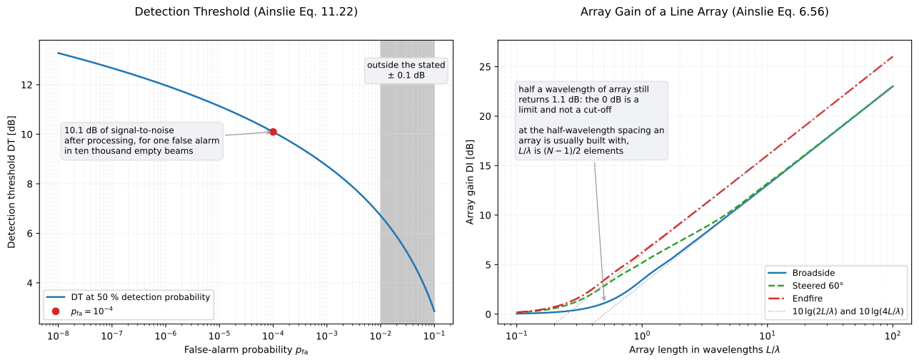
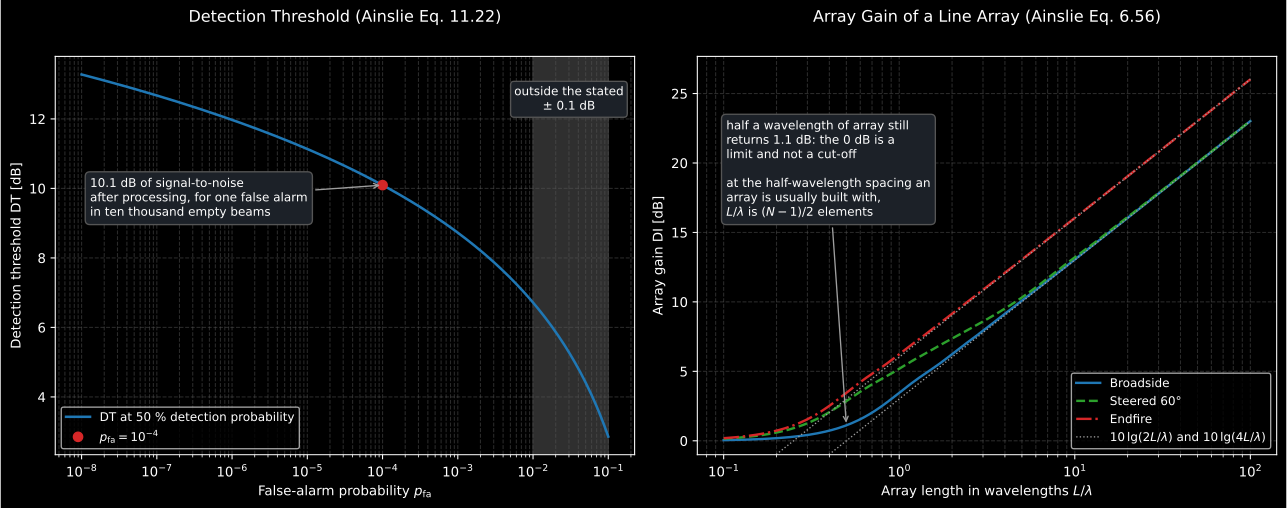
The two terms the receiver contributes, each over the one variable it depends on. Neither is measured at sea: the threshold is a property of the detector and the gain one of the array, and a design choice in each moves the figure of merit decibel for decibel. The approximation is drawn past the the book states it to, because the reader who works there should see what the formula gives and that it is an extrapolation. On the right the three steer directions share one limit and not one asymptote: the beam’s footprint halves near endfire, which is the 3 dB between the two dotted lines, and the whole family flattens to 0 dB rather than cutting off, a half-wavelength array still returning 1.1 dB.
Detection range
Section titled “Detection range”Since the figure of merit is the maximum allowable propagation loss,
inverting a loss law at gives the detection range, the range at
which the detection probability is 50 %. detection_range inverts the
closed-form loss above, which grows monotonically with range and therefore has
a single crossing; detection_range_from_curve reads the crossing off any
computed curve, including the oscillating loss of a real waveguide where there
may be several.
from phonometry import underwater
# Ainslie's active CW example: FOM = 82.7 dB re m2 at 50 kHz -> r50 ~ 1.3 km.res = underwater.detection_range(82.7, 50e3)print(res.detection_range)          # metresres.plot()                          # PL vs FOM with the crossing marked
That call carries four silent defaults: law="spherical", 10 °C, 35 ppt and
surface depth, with Francois-Garrison absorption. The spreading assumption alone
moves the answer by nearly a factor of two, so it is a choice to make
deliberately rather than one to inherit. At 50 kHz, where absorption
dominates, the temperature and depth passed to it are not decorative either.
Reach for detection_range_from_curve whenever the loss came from a solver
instead of a law.
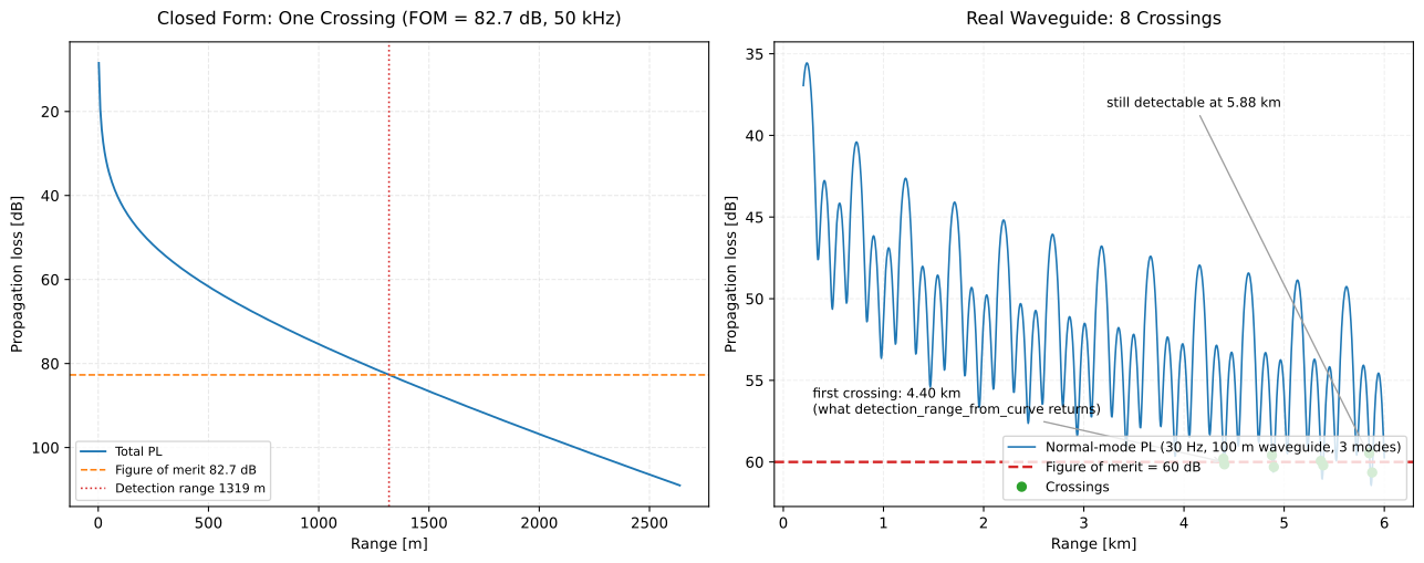
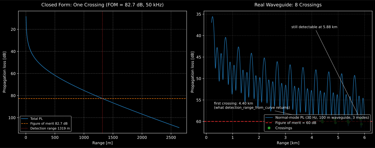
The closed-form loss grows monotonically, so the crossing is unique and
detection_range can return it. A real waveguide’s loss oscillates: here the
same figure of merit is crossed eight times between 4 and 6 km, and
detection_range_from_curve returns the first of them, 4.4 km, by default.
The loss dips back under the figure of merit as far out as 5.9 km, so quoting
4.4 km as “the” detection range is a convention rather than a fact, and it needs
saying in the report.
Show the code for this figure
import matplotlib.pyplot as pltimport numpy as np
fig, (ax_c, ax_m) = plt.subplots(1, 2, figsize=(13.5, 5.4))underwater.detection_range(82.7, 50e3).plot(ax=ax_c)
ranges = np.linspace(200.0, 6000.0, 1200)modes = underwater.normal_modes(30.0, [0.0, 100.0], [1500.0, 1500.0],                                source_depth=25.0, receiver_depth=60.0,                                ranges_m=ranges, n_depth_points=800)pl = np.asarray(modes.propagation_loss)ax_m.plot(ranges / 1000.0, pl, label="Normal-mode PL (30 Hz, 100 m)")ax_m.axhline(60.0, linestyle="--", label="Figure of merit = 60 dB")print(underwater.detection_range_from_curve(60.0, ranges, pl))   # first crossingax_m.invert_yaxis()ax_m.set(xlabel="Range [km]", ylabel="Propagation loss [dB]")ax_m.legend()plt.show()
Seabed reflection loss
Section titled “Seabed reflection loss”A plane wave striking the seabed reflects with the fluid–fluid Rayleigh reflection coefficient (Medwin & Clay). For a faster bottom () there is a critical grazing angle : the same that fixes the Weston regime boundaries above, below which the wave is totally reflected (, zero loss). The bottom loss is .
Total reflection below is a property of the lossless fluid-fluid idealisation, not of any real sea floor. A real sediment absorbs, so sits a little under one at every angle, and in shallow water that small difference is the whole answer: a ray reaches long range only after many bounces, so a few hundredths of a decibel per reflection accumulate into the dominant range dependence. That accumulated quantity is exactly what the Weston reflection loss gradient parameterises. Read the two together: the Rayleigh curve locates the critical angle and the shape of the loss above it, while the Weston gradient answers how far sound gets.
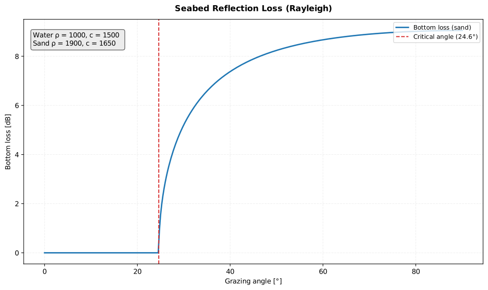
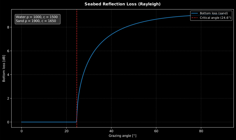
A ray that stays shallow pays nothing, and a steep one pays almost everything. For this water-over-sand pair the critical angle is 24.62°: below it the loss is identically zero, and one degree above it the curve is already climbing, through 5.21 dB at 30°, 7.89 dB at 45° and 9.05 dB at normal incidence. That step is what makes shallow-water propagation an angle-filtering problem, after a few bounces only the sub-critical rays survive, which is the mode stripping the Weston regimes describe.
Show the code for this figure
import matplotlib.pyplot as pltimport numpy as npfrom phonometry import underwater
# Rayleigh fluid-fluid reflection: water over a fast sandy bottom.psi = np.linspace(0.0, 90.0, 361)bl = underwater.bottom_reflection_loss(psi, rho1=1000.0, c1=1500.0,                                       rho2=1900.0, c2=1650.0)print(f"critical angle = {bl.critical_angle_deg:.1f} deg")   # critical angle = 24.6 degbl.plot()   # bottom loss vs grazing angleplt.show()
import numpy as npfrom phonometry import underwater
psi = np.linspace(0.0, 90.0, 361) # grazing angle from the interface, degreesbl = underwater.bottom_reflection_loss(psi, rho1=1000.0, c1=1500.0, # water rho2=1900.0, c2=1650.0) # sandprint(bl.critical_angle_deg) # 24.6°bl.plot() # bottom loss vs grazing angle (needs matplotlib)The companion seabed_reflection bundles the complex reflection_coefficient,
its magnitude , the bottom_loss (dB) and the interface parameters into a
SeabedReflection whose .plot() draws the reflection-coefficient magnitude
directly (unity below the critical angle, dropping to the normal-incidence
value at ).
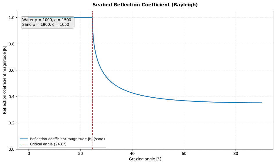
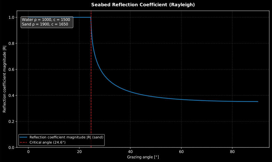
The same interface as the loss above, read as an amplitude. is exactly 1 out to 24.62°, then falls fast, 0.403 at 45° and 0.353 at normal incidence, the plane-wave impedance ratio of the two media. The lossless idealisation is what makes the sub-critical part flat: a real absorbing sediment pulls it a few hundredths below one, which is invisible on this axis and is the dominant term after fifty bounces.
Show the code for this figure
import matplotlib.pyplot as pltimport numpy as npfrom phonometry import underwater
# Rayleigh reflection-coefficient magnitude: water over a fast sandy bottom.psi = np.linspace(0.0, 90.0, 361)sr = underwater.seabed_reflection(psi, rho1=1000.0, c1=1500.0,                                  rho2=1900.0, c2=1650.0)print(f"|R| at normal incidence = {sr.magnitude[-1]:.3f}")  # 0.353sr.plot()   # reflection-coefficient magnitude vs grazing angleplt.show()
import numpy as npfrom phonometry import underwater
psi = np.linspace(0.0, 90.0, 361) # grazing angle from the interface, degreessr = underwater.seabed_reflection(psi, rho1=1000.0, c1=1500.0, # water rho2=1900.0, c2=1650.0) # sandprint(sr.magnitude[-1]) # 0.353 = |R| at normal incidencesr.plot() # |R| vs grazing angle (needs matplotlib)The same interface, as a field
Section titled “The same interface, as a field”Both curves above are read at one angle at a time, and the seabed is never struck at one angle: a source radiates every angle at once, and which of them strikes where is geometry. The clip below builds that geometry from a single 100 Hz burst 36 m above the bed. Its expanding front touches the seabed directly beneath the source at and the contact point then runs outward, sweeping the grazing angle down through 24.62° and on to a few degrees at the edge of the frame, so the whole curve is traversed once, in order, in a single shot. The scene is then run twice, changing nothing but the two numbers that describe the sediment.
A 100 Hz burst 36 metres above a flat seabed, simulated twice: over the fast sand of the figures above and over a slow mud. As the expanding front's contact with the bed sweeps outward the grazing angle falls, and over the sand the beam entering the sediment switches off where the 24.62 degree critical ray meets the bed, leaving only a bright evanescent skin that carries nothing away; over the mud sound enters at every angle right to the edge of the frame. A lower axis fills in the measured net energy flux through the seabed behind the contact point and lands on the closed form.
A 100 Hz burst 36 metres above a flat seabed, simulated twice: over the fast sand of the figures above and over a slow mud. As the expanding front's contact with the bed sweeps outward the grazing angle falls, and over the sand the beam entering the sediment switches off where the 24.62 degree critical ray meets the bed, leaving only a bright evanescent skin that carries nothing away; over the mud sound enters at every angle right to the edge of the frame. A lower axis fills in the measured net energy flux through the seabed behind the contact point and lands on the closed form.
Over the sand, transmission ends at the critical ray and what is left in the sediment is an evanescent skin: bright, and carrying nothing away. Measured on the interface itself, the net per metre of seabed, which an evanescent field contributes nothing to, the sand’s net beyond the critical ray is −4.9 % of what entered inside it, against 0 % from the closed form, and the sign is not a rounding error: past the critical range the net flux reverses, because the lateral wave born at the critical point runs along the interface inside the sediment and radiates back up into the water. The mud takes +28.3 % beyond that same range against +29.7 % predicted, and its curve simply carries on falling off the right of the panel. That difference, paid again at every bounce, is what the Weston reflection loss gradient accumulates.
Two things the clip deliberately does not show. There is no sea surface in it: with one interface the picture has one family of rays and one critical range, whereas a real waveguide adds a surface-reflected family whose image sits higher and whose own critical range is further out. And it is a single bounce, so the angle filtering is visible but the accumulation over many bounces (the mode stripping of the Weston table) is not. That is the quantity stands in for.
Ocean ambient noise
Section titled “Ocean ambient noise”The ambient-noise spectrum level is the energy sum of the physically grounded Wenz components: wind / sea-surface noise via the “rule of fives” (the historical 25 dB anchor at 1 kHz for 5 knots is re 20 µPa, i.e. ~51 dB re 1 µPa; strictly valid ~500 Hz–5 kHz) and Mellen thermal noise (dominant above ~50 kHz). The wide example range keeps the wind curve plotted beyond ~5 kHz only as an extrapolation to show the thermal crossover. A shipping spectrum may be supplied by the caller.
The “rule of fives” is a mnemonic worth unpacking, because it is where the whole
wind branch comes from: about 5 dB per octave of falloff, anchored at a 5 knot
wind and 1 kHz, where the historical figure is 25 dB re 20 µPa. Hence
ocean_ambient_noise returns 51 dB re 1 µPa²/Hz there. Read the spectrum
in three bands. Below a couple of hundred hertz a real site is normally owned by
shipping, which this model leaves to the caller, so the wind curve there is a
floor and not a prediction. Between a few hundred hertz and a few kilohertz wind
noise genuinely dominates and the model earns its keep: at 1 kHz it gives 51 dB
at 5 knots against 64 dB in a 30 knot gale, so wind speed is the one knob and it
moves the mid band by more than a decade of sea state. Above tens of kilohertz
nothing beats Mellen thermal noise, which sets the absolute floor of any
hydrophone measurement: 25 dB re 1 µPa²/Hz at 100 kHz, wind or no wind. A
composite total outside roughly 30-100 dB re 1 µPa²/Hz over 100 Hz to 100 kHz is
an input error rather than an unusual ocean.
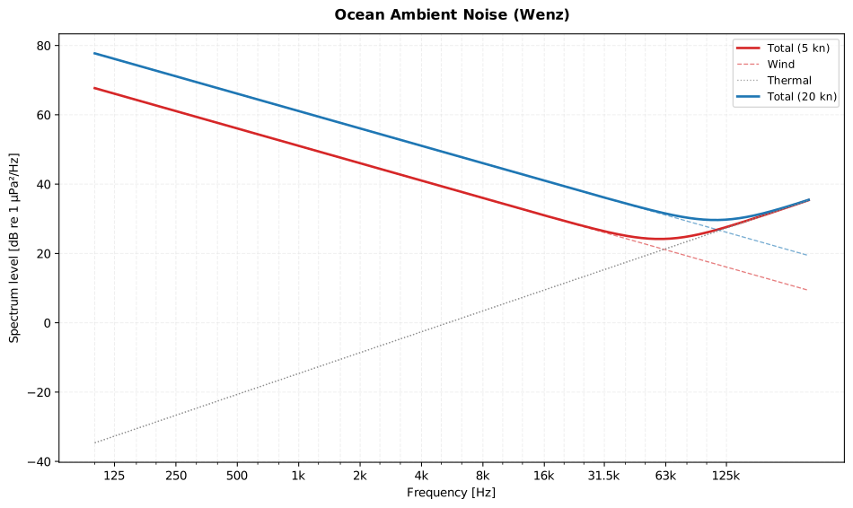
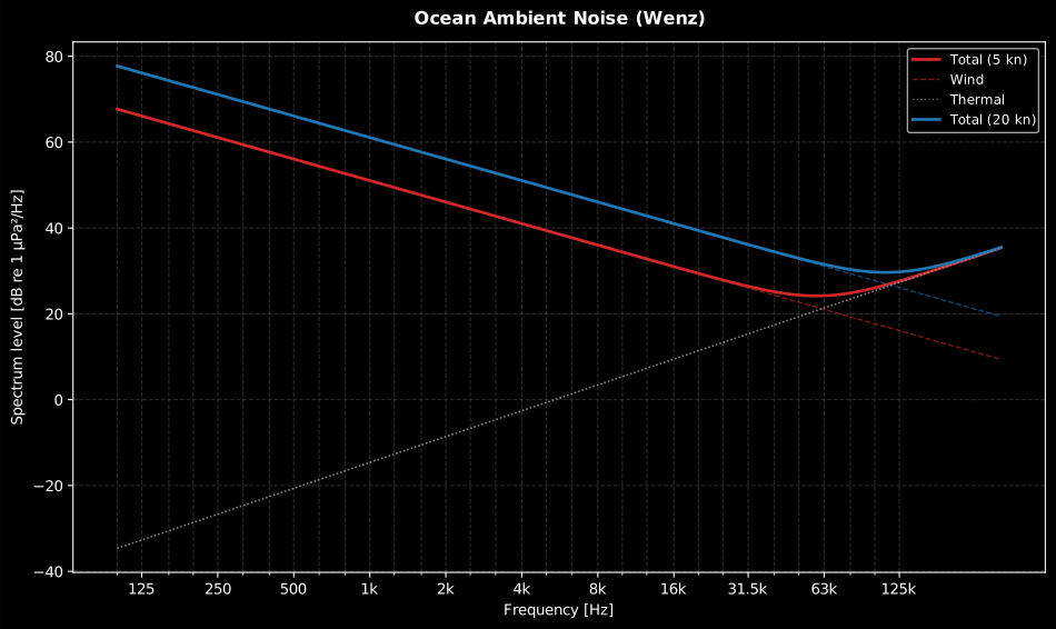
The rule of fives, measured: between 500 Hz and 5 kHz the wind branch falls 5.02 dB per octave, and going from 5 to 20 knots lifts it by 10.03 dB at 1 kHz: 51.1 dB against 61.1 dB. The two mechanisms then run in opposite directions, so the total has a minimum: thermal noise reaches 25.3 dB at 100 kHz and at 5 knots is already within 0.7 dB of the total there, while at 20 knots the wind still wins. Nothing on this figure is a floor a quieter hydrophone could get below: the thermal branch is the water itself.
Show the code for this figure
import matplotlib.pyplot as pltimport numpy as npfrom phonometry import underwater
# Wenz ambient noise (wind rule of fives + Mellen thermal) at two wind speeds.freqs = np.logspace(2, 5.5, 300)fig, ax = plt.subplots()for u in (5.0, 20.0):    noise = underwater.ocean_ambient_noise(freqs, wind_speed_knots=u)    ax.semilogx(noise.frequencies, noise.spectrum_level, label=f"Total ({u:.0f} kn)")ax.semilogx(freqs, underwater.thermal_noise_spectrum(freqs), ":", label="Thermal")ax.set(xlabel="Frequency [Hz]", ylabel="Spectrum level [dB re 1 µPa²/Hz]")ax.legend()ax.grid(True, which="both", alpha=0.3)plt.show()
import numpy as npfrom phonometry import underwater
freqs = np.logspace(2, 5.5, 300)noise = underwater.ocean_ambient_noise(freqs, wind_speed_knots=15.0)noise.plot() # composite spectrum with wind/thermal components (needs matplotlib)Ship-traffic source level
Section titled “Ship-traffic source level”When no measured spectrum is available, a ship’s source level can be estimated from its class, speed and length with JOMOPANS-ECHO (MacGillivray & de Jong 2021, the default, validated against 1862 measurements), RANDI 3.1 or Wales & Heitmeyer (2002).
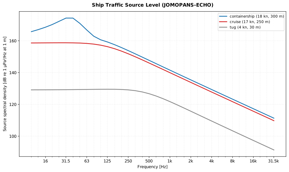
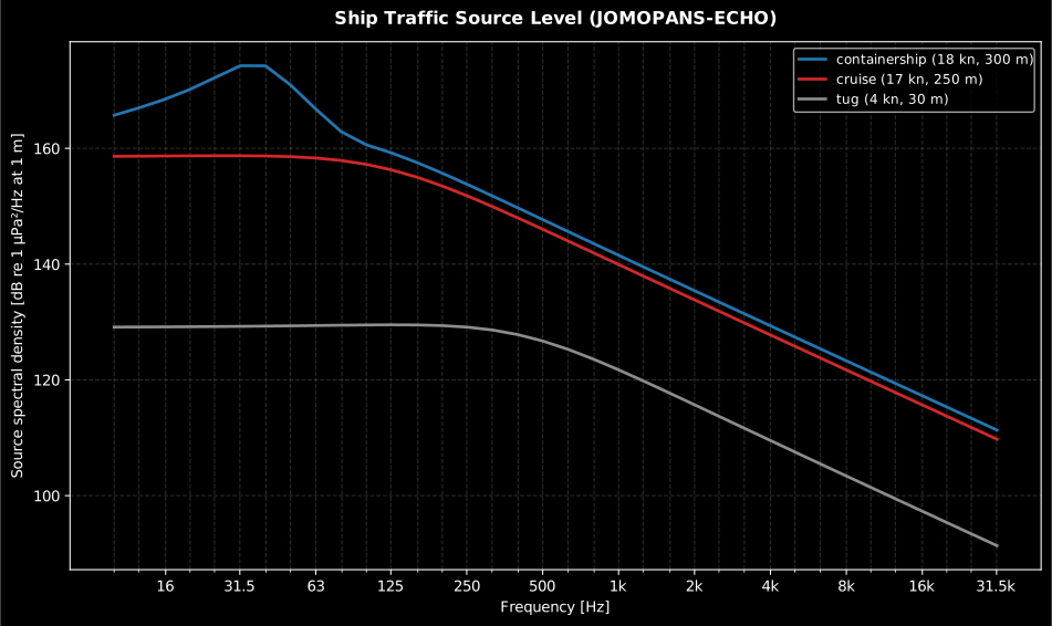
Class, speed and length are the only inputs, and they span 45 dB. The containership peaks at 174.3 dB re 1 µPa²/Hz at 31.6 Hz, the cruise ship at 158.7 dB at 25.1 Hz, and the tug (slow and short) at 129.5 dB and up at 125.9 Hz. Two things follow: the fleet’s energy is below 100 Hz, which is where the wind model of the previous section is weakest, and a single number for “shipping noise” is meaningless without the class. These are source levels at 1 m; the snippet below shows what forgetting that costs.
Show the code for this figure
import matplotlib.pyplot as pltfrom phonometry import underwater
# JOMOPANS-ECHO source spectra for three vessel classes (speed, length).fig, ax = plt.subplots()for vessel_class, speed, length in (("containership", 18.0, 300.0),                                    ("cruise", 17.1, 250.0),                                    ("tug", 3.7, 30.0)):    s = underwater.ship_source_spectrum(speed, length, vessel_class=vessel_class)    ax.semilogx(s.frequencies, s.source_psd,                label=f"{vessel_class} ({speed:.0f} kn, {length:.0f} m)")ax.set(xlabel="Frequency [Hz]",       ylabel="Source spectral density [dB re 1 µPa²/Hz at 1 m]")ax.legend()ax.grid(True, which="both", alpha=0.3)plt.show()
import numpy as npfrom phonometry import underwater
ship = underwater.ship_source_spectrum(18.0, 300.0, vessel_class="containership")ship.plot() # source spectral density vs frequencyprint(underwater.VESSEL_CLASSES) # the 13 JOMOPANS-ECHO vessel classes
# `source_psd` is a SOURCE level at 1 m; the `shipping` term of the ambient sum# is a RECEIVED spectrum level at the listening position. Propagation is the# step between them - here that one ship, 2 km away.pl = np.array([float(underwater.propagation_loss( 2000.0, float(f), law="practical", transition_range=1000.0).pl[0]) for f in ship.frequencies])received = ship.source_psd - plnoise = underwater.ocean_ambient_noise(ship.frequencies, wind_speed_knots=10.0, shipping=received)print(round(float(np.interp(100.0, ship.frequencies, noise.spectrum_level)), 1))# 97.6 dB re 1 uPa^2/Hz at 100 Hz, against 72.7 for the wind alone. Passing# ship.source_psd straight in would print 160.6: a source level is not a# received one, and the error is the whole propagation loss.Even that is a single-ship estimate. Measured shipping noise at a site is the
sum over the whole traffic field, so a realistic term integrates many vessels
over their ranges and classes, which is why ocean_ambient_noise leaves the
shipping spectrum to the caller instead of building one in. One sanity check
carries most of the value: a composite ambient spectrum above roughly
120 dB re 1 µPa²/Hz is a units or geometry error, not a noisy sea.
Every closed form above stops being enough when refraction and boundaries decide the answer: a sound-speed minimum that traps energy, surface and bottom reflections in shallow water, or a detection range that swings with the choice of spreading law. At that point the field has to be computed, and the normal-mode, ray-tracing, Gaussian-beam and parabolic-equation solvers of the module, together with the guidance for choosing between them and these closed forms, have their own guide: Underwater propagation solvers.
What this guide covers
Section titled “What this guide covers”Covered
ISO 18405:2017 terminology (propagation loss, source level, levels re 1 µPa) underlies every quantity on this page.
propagation_lossandseawater_absorptionimplement geometrical spreading plus the Francois-Garrison (1982, default), Ainslie-McColm (1998) or Thorp (1967) absorption models.sea_water_sound_speedandsound_speed_profileimplement the UNESCO/Chen-Millero (Wong & Zhu 1995 ITS-90 form, default), Del Grosso (1974), Mackenzie (1981) and Medwin (1975) sound-speed equations, with the Leroy & Parthiot (1998) depth-to-pressure conversion.weston_propagation_lossandweston_regime_boundariesimplement the four Weston energy-flux regimes and their transition ranges (Ainslie section 9.1.1.2, Table 9.1).passive_sonar_equationandactive_sonar_equationimplement the passive and monostatic active sonar equations (Urick, via Etter 2003), anddetection_range/detection_range_from_curveinvert a propagation loss at the figure of merit.seabed_reflectionandbottom_reflection_lossimplement the fluid-fluid Rayleigh reflection coefficient and critical angle (Medwin & Clay).ocean_ambient_noisesums the Wenz wind “rule of fives” and Mellen thermal-noise components.ship_source_spectrumimplements the JOMOPANS-ECHO (default), RANDI 3.1 and Wales & Heitmeyer (2002) source-level models.Not covered
The seabed model is lossless fluid-fluid Rayleigh reflection only, so sediment attenuation is out of scope.
active_sonar_equationis monostatic only: there is no bistatic geometry.ocean_ambient_noiseleaves out the low-frequency turbulence band and any built-in distant-shipping model; supply a shipping spectrum yourself, for instance fromship_source_spectrumabove. The numerical field solvers (normal_modes,ray_trace,gaussian_beams,parabolic_equation) are covered in Underwater propagation solvers.
References
Section titled “References”- Ainslie, M. A. (2010). Principles of Sonar Performance Modelling. Springer/Praxis. https://doi.org/10.1007/978-3-540-87662-5The Weston shallow-water propagation regimes (section 9.1.1.2, Equations 9.42 to 9.61 and Table 9.1), the Medwin sound-speed formula (Equation 1.2) and the seven numeric sonar worked examples of chapters 3 and 11 that pin the sonar-equation section.
- Ainslie, M. A., & McColm, J. G. (1998). A simplified formula for viscous and chemical absorption in sea water. The Journal of the Acoustical Society of America, 103(3), 1671-1672. https://doi.org/10.1121/1.421258The legible simplified absorption model ("ainslie-mccolm").
- Carey, W. M., & Evans, R. B. (2011). Ocean ambient noise: Measurement and theory. Springer. https://doi.org/10.1007/978-1-4419-7832-5The wind "rule of fives" anchor and the Mellen thermal-noise derivation.
- Chen, C.-T., & Millero, F. J. (1977). Speed of sound in seawater at high pressures. The Journal of the Acoustical Society of America, 62(5), 1129-1135. https://doi.org/10.1121/1.381646The UNESCO international-standard sound-speed equation.
- Del Grosso, V. A. (1974). New equation for the speed of sound in natural waters (with comparisons to other equations). The Journal of the Acoustical Society of America, 56(4), 1084-1091. https://doi.org/10.1121/1.1903388The alternative pressure-based sound-speed equation ("del_grosso").
- Francois, R. E., & Garrison, G. R. (1982). Sound absorption based on ocean measurements: Part I: Pure water and magnesium sulfate contributions. The Journal of the Acoustical Society of America, 72(3), 896-907. https://doi.org/10.1121/1.388170The pure-water and magnesium-sulfate halves of the default absorption model of the propagation-loss section.
- Francois, R. E., & Garrison, G. R. (1982). Sound absorption based on ocean measurements. Part II: Boric acid contribution and equation for total absorption. The Journal of the Acoustical Society of America, 72(6), 1879-1890. https://doi.org/10.1121/1.388673The boric-acid term and the complete Francois-Garrison total-absorption equation, the implemented default.
- International Organization for Standardization. (2017). Underwater acoustics — Terminology (ISO 18405:2017). The standardized definitions (propagation loss, source level, sound pressure level re 1 µPa) behind the quantities of this page.
- Leroy, C. C., & Parthiot, F. (1998). Depth-pressure relationships in the oceans and seas. The Journal of the Acoustical Society of America, 103(3), 1346-1352. https://doi.org/10.1121/1.421275The depth-to-pressure conversion feeding the UNESCO and Del Grosso equations.
- MacGillivray, A., & de Jong, C. (2021). A reference spectrum model for estimating source levels of marine shipping based on automated identification system data. Journal of Marine Science and Engineering, 9(4), 369. https://doi.org/10.3390/jmse9040369The JOMOPANS-ECHO ship source-level model (open access); its File S1 calculator is the validation oracle.
- Mackenzie, K. V. (1981). Nine-term equation for sound speed in the oceans. The Journal of the Acoustical Society of America, 70(3), 807-812. https://doi.org/10.1121/1.386920The depth-based nine-term equation and its 1550.744 m/s check value.
- Medwin, H., & Clay, C. S. (1998). Fundamentals of acoustical oceanography. Academic Press. ISBN 978-0-12-487570-8. The fluid-fluid Rayleigh reflection coefficient and critical grazing angle of the seabed-reflection section.
- Thorp, W. H. (1967). Analytic description of the low-frequency attenuation coefficient. The Journal of the Acoustical Society of America, 42(1), 270. https://doi.org/10.1121/1.1910566The frequency-only low-frequency absorption formula ("thorp").
- Urick, R. J. (1983). Principles of underwater sound (3rd ed.). McGraw-Hill. Reprinted 1996 by Peninsula Publishing. ISBN 978-0-932146-62-5. Open Library record (https://openlibrary.org/books/OL9317725M). The sonar-equation framework (signal excess, figure of merit).
- Wales, S. C., & Heitmeyer, R. M. (2002). An ensemble source spectra model for merchant ship-radiated noise. The Journal of the Acoustical Society of America, 111(3), 1211-1231. https://doi.org/10.1121/1.1427355The ensemble merchant-ship spectrum model of the ship-traffic section.
- Wenz, G. M. (1962). Acoustic ambient noise in the ocean: Spectra and sources. The Journal of the Acoustical Society of America, 34(12), 1936-1956. https://doi.org/10.1121/1.1909155The ambient-noise survey behind the wind and thermal components of the ocean ambient-noise section.
- Wong, G. S. K., & Zhu, S. (1995). Speed of sound in seawater as a function of salinity, temperature, and pressure. The Journal of the Acoustical Society of America, 97(3), 1732-1736. https://doi.org/10.1121/1.413048The ITS-90 recast of the UNESCO coefficients, the implemented form.