Underwater propagation solvers

The closed-form propagation loss of Underwater sound propagation knows nothing of the sound-speed profile, the seabed or the surface. When refraction and boundaries decide the answer, the field has to be computed: this guide covers the four numerical solvers of the underwater module, the physics each one discretises, and how to choose between them and the closed forms. All four take the same range-independent (horizontally stratified) $c(z)$ profile and a pressure-release surface, and follow Jensen, Kuperman, Porter & Schmidt, Computational Ocean Acoustics; the two ray-based solvers can also slope the bottom over a piecewise-linear depth profile (section 3), the one range dependence in the module.

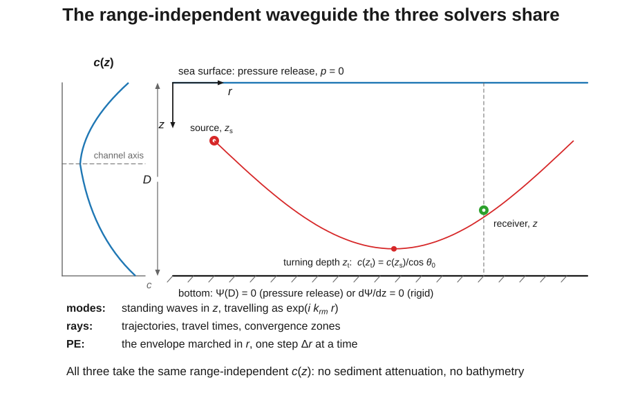
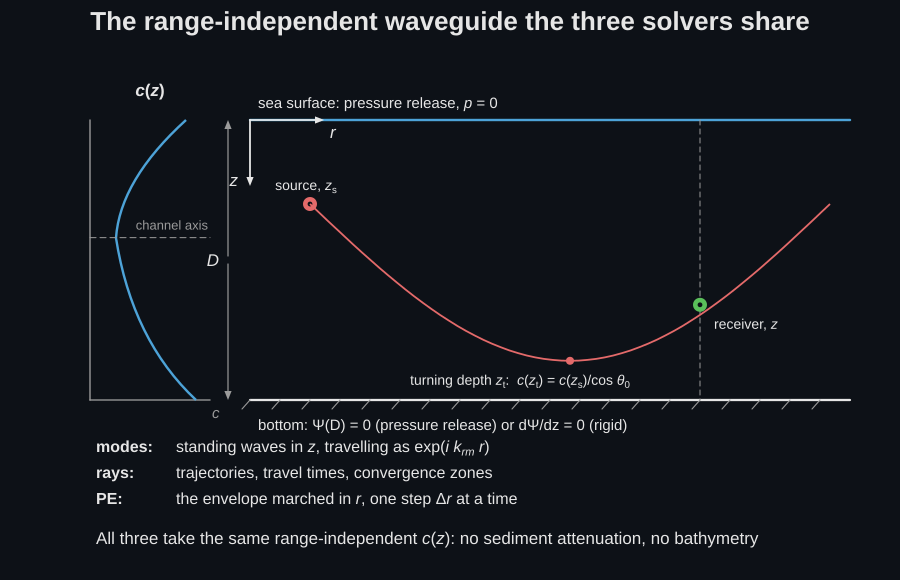
• normal_modes solves the depth-separated Sturm-Liouville eigenvalue problem by finite differences and sums the propagating modes into the propagation loss. Validated against the ideal (pressure-release) waveguide’s exact modes.
• ray_trace integrates the ray-trajectory equations (Runge-Kutta, vectorised over all rays at once) through a sound-speed profile, reflecting at the surface and bottom, and carries the travel time along each ray as a state of the same integration. Validated against the circular-arc paths of a linear gradient and the closed-form travel time along them. eigenrays then searches that traced fan for the paths that join the source to one receiver and lists their arrivals, validated against the image lattice of the ideal waveguide, where every arrival is closed form.
• gaussian_beams hangs a Gaussian beam on each of those rays and sums them into a propagation-loss field, which stays finite at the caustics where the classical ray amplitude is infinite and decays into the shadow zones where it is not defined at all. Validated against free-field spherical spreading, the two-ray Lloyd-mirror field and the image-source sum of the ideal waveguide.
• parabolic_equation marches the standard (Tappert) PE with the split-step Fourier algorithm. Validated against free-field spherical spreading; it agrees with the normal-mode propagation loss in trend.

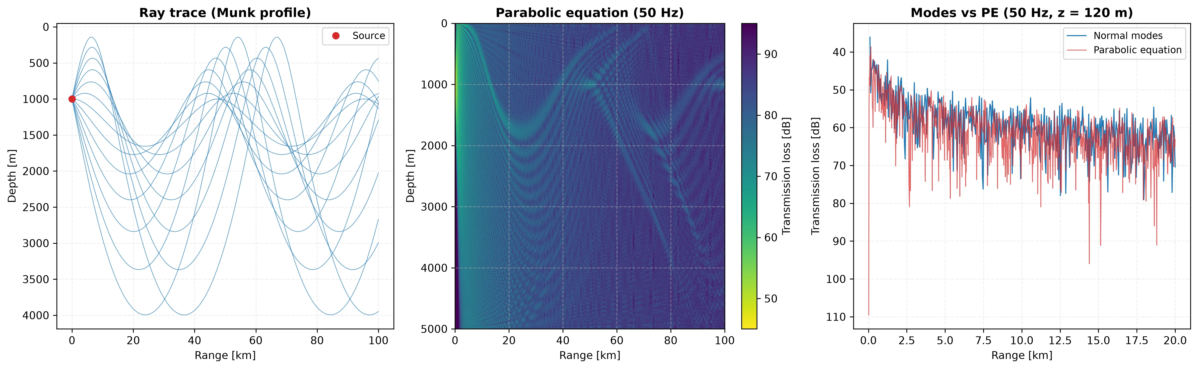
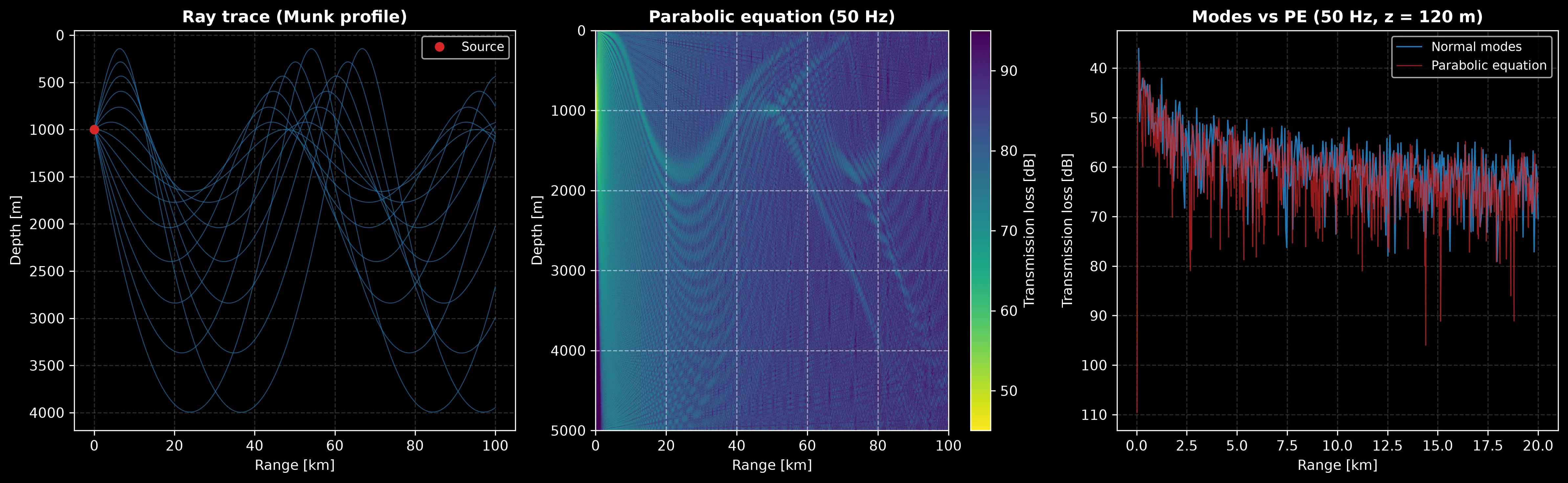
Three panels, three different questions about the same water. Left, rays in a Munk profile whose minimum is 1500.0 m/s at 1271 m against 1548.5 m/s at the surface: a 48 m/s spread is enough to fold the ±12° fan back on itself into convergence zones, and the ±12° ray still sweeps from 143 m to 3997 m of depth. Centre, the same environment as a PE field, where the zones appear as interference rather than as lines. Right, the two solvers on a different, 200 m shallow waveguide: they track the same trend with a mean offset of 1.6 dB, but the per-range difference reaches 25 dB at the interference nulls, which is the honest statement of what “agree in trend” means.

import matplotlib.pyplot as plt
import numpy as np
from phonometry import underwater

# A Munk deep-water sound-speed profile for the ray and PE panels.
z = np.linspace(0.0, 5000.0, 60)
eta = 2.0 * (z - 1300.0) / 1300.0
c = 1500.0 * (1.0 + 0.00737 * (eta - 1.0 + np.exp(-eta)))

fig, axes = plt.subplots(1, 3, figsize=(16, 5))

# (a) rays through the Munk profile, out to 100 km.
underwater.ray_trace(z, c, source_depth=1000.0,
                     launch_angles_deg=np.linspace(-12.0, 12.0, 13),
                     max_range=100e3, n_steps=6000).plot(ax=axes[0])

# (b) the split-step Fourier PE field over the same environment.
underwater.parabolic_equation(50.0, z, c, source_depth=1000.0,
                              max_range=100e3, range_step=25.0,
                              n_depth_points=1024).plot(ax=axes[1])

# (c) modes against PE in a *different*, shallow 200 m waveguide.
r = np.linspace(100.0, 20_000.0, 400)
nm = underwater.normal_modes(50.0, [0.0, 200.0], [1500.0, 1530.0],
                             source_depth=30.0, receiver_depth=120.0,
                             ranges_m=r, n_depth_points=800)
pe = underwater.parabolic_equation(50.0, [0.0, 200.0], [1500.0, 1530.0],
                                   source_depth=30.0, max_range=20e3,
                                   range_step=20.0, n_depth_points=512)
zi = int(np.argmin(np.abs(pe.depths - 120.0)))
axes[2].plot(nm.ranges / 1000.0, nm.propagation_loss, label="Normal modes")
axes[2].plot(pe.ranges / 1000.0, pe.propagation_loss[zi], label="PE")
axes[2].invert_yaxis()
axes[2].set(xlabel="Range [km]", ylabel="Propagation loss [dB]")
axes[2].legend()
plt.show()

import numpy as np
from phonometry import underwater

# A Munk deep-water profile.
z = np.linspace(0.0, 5000.0, 60)
eta = 2.0 * (z - 1300.0) / 1300.0
c = 1500.0 * (1.0 + 0.00737 * (eta - 1.0 + np.exp(-eta)))

rays = underwater.ray_trace(z, c, source_depth=1000.0,
                    launch_angles_deg=np.linspace(-12.0, 12.0, 21), max_range=100e3)
rays.plot()   # ray paths / convergence zones (needs matplotlib)

# Shallow isovelocity waveguide: modes and PE.
modes = underwater.normal_modes(50.0, [0.0, 200.0], [1500.0, 1500.0],
                        source_depth=50.0, receiver_depth=100.0)
print(modes.wavenumbers.size, "propagating modes")
field = underwater.parabolic_equation(50.0, [0.0, 200.0], [1500.0, 1500.0],
                              source_depth=50.0, max_range=20e3)
field.plot()  # PL field over range x depth (needs matplotlib)

normal_modes returns a NormalModeResult (wavenumbers, mode_functions, propagation_loss); ray_trace a RayTraceResult (ranges, depths, travel_times, arc_lengths and per-boundary reflection counts per ray); gaussian_beams a GaussianBeamResult (the propagation_loss field, plus each beam’s central ray and width); parabolic_equation a ParabolicEquationResult (the propagation_loss field). The four differ in what they model, so choosing between them is a regime question — the table in section 6 is the short answer.

In a horizontally stratified ocean the Helmholtz equation separates in cylindrical coordinates, $p(r,z)=\Phi (r)\Psi (z)$, and the depth factor obeys a Sturm-Liouville eigenvalue problem (Jensen Eq. 5.3):

with a pressure-release surface at $z=0$ and, at the bottom $z=D$, $\Psi (D)=0$ for a pressure-release bed or $d\Psi /dz{|}_D=0$ for a rigid one. Each eigenfunction ${\Psi }_m(z)$ is a standing wave in depth that travels in range as $e^{i{k}_{rm}r}$ with its own horizontal wavenumber $k_{rm}$; only the modes with real $k_{rm}$ propagate, the rest are evanescent and die within a few water depths. The field is the modal sum (Eq. 5.14),

each mode weighted by its excitation at the source depth ${\Psi }_m(z_{\mathrm{s}})$ and its amplitude at the receiver depth ${\Psi }_m(z)$, and the coherent propagation loss follows as $PL=-20{\log }_{10}|p(r,z)/p_0(1\mathrm{m})|$ (Eq. 5.15). normal_modes discretises the depth equation by finite differences (a symmetric tridiagonal eigenproblem) on a grid refined enough to keep the near-cutoff eigenvalues honest, and warns when a retained mode sits too close to its discretisation error band.

The mode count is the physics: an isovelocity channel of depth $D$ carries $M\approx kD/\pi$ propagating modes, so a 200 m channel at 50 Hz carries 13 and the same channel at 5 kHz would carry over 1300 — which is the frequency at which rays become the economical description. Low frequency and shallow water mean few modes and a compact, essentially exact description. The ideal pressure-release waveguide is the validation oracle, with $k_{rm}=\sqrt{k^2-(m\pi /D{)}^2}$ in closed form:

import numpy as np
from phonometry import underwater

# A 200 m isovelocity channel at 50 Hz: kD/pi = 2 f D / c = 13.3.
modes = underwater.normal_modes(50.0, [0.0, 200.0], [1500.0, 1500.0],
                                source_depth=50.0, receiver_depth=100.0)
print(modes.wavenumbers.size)                   # 13  propagating modes
k = 2 * np.pi * 50.0 / 1500.0
print(round(float(modes.wavenumbers[0]), 5))    # 0.20885  computed kr1
print(round(np.sqrt(k**2 - (np.pi / 200.0) ** 2), 5))   # 0.20885  exact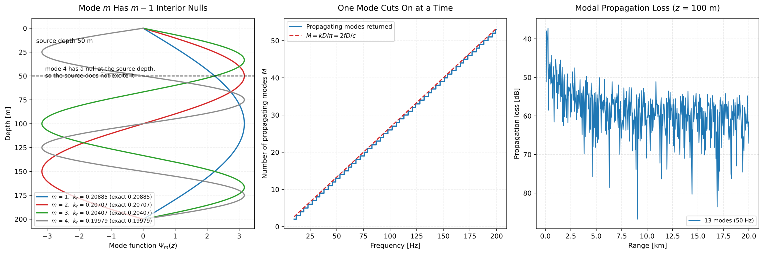

Mode $m$ has $m-1$ interior nulls, and the source depth decides which modes exist in the field at all: the fourth mode has a null at exactly 50 m in a 200 m channel, so a source there does not excite it. The staircase in the middle is the mode count cutting on one mode at a time as frequency rises, tracking $M\approx kD/\pi$; the right-hand panel is the interference of the 13 modes that survive at 50 Hz. A computed result draws all three with modes.plot().

import matplotlib.pyplot as plt
import numpy as np

fig, axes = plt.subplots(1, 3, figsize=(16, 5.4))
r = np.linspace(100.0, 20_000.0, 500)
res = underwater.normal_modes(50.0, [0.0, 200.0], [1500.0, 1500.0],
                              source_depth=50.0, receiver_depth=100.0,
                              ranges_m=r, n_depth_points=800)
for m in range(4):
    axes[0].plot(res.mode_functions[m], res.mode_depths, label=f"m = {m + 1}")
axes[0].axhline(50.0, linestyle="--")
axes[0].invert_yaxis()
axes[0].set(xlabel="Mode function Psi_m(z)", ylabel="Depth [m]")
axes[0].legend()

freqs = np.arange(10.0, 201.0, 1.0)
counts = [underwater.normal_modes(f, [0.0, 200.0], [1500.0, 1500.0],
                                  source_depth=50.0, receiver_depth=100.0,
                                  n_depth_points=1200).wavenumbers.size
          for f in freqs]
axes[1].step(freqs, counts, where="post", label="modes returned")
axes[1].plot(freqs, 2.0 * freqs * 200.0 / 1500.0, "--", label="M = kD/pi")
axes[1].set(xlabel="Frequency [Hz]", ylabel="Propagating modes M")
axes[1].legend()

res.plot(ax=axes[2])
plt.show()

That ideal waveguide plays two roles, and they should not be confused. It is the exact oracle the solver is checked against — which is why it is used here — and it is also a physically extreme bottom: a pressure-release bed reflects with unit magnitude and a phase inversion, so it transmits nothing into the sediment and absorbs nothing. A modal or PE propagation loss computed over it therefore understates the loss of any real seabed, and the gap widens with range because it accumulates over bounces. The rigid option is the opposite extreme, offered for the same validation reason and not as a sediment model. For a real bottom in shallow water, price the seabed with the Weston regimes of Underwater sound propagation, whose critical angle and reflection-loss gradient encode exactly what these boundary conditions omit, and read the modal answer as an upper bound on the received level. Or hand gaussian_beams the fluid seabed itself (section 4), which charges every bottom bounce with the Rayleigh coefficient these two extremes idealise away.

In the high-frequency limit the Helmholtz equation collapses to the eikonal equation, and its characteristics are rays: trajectories integrated from the first-order system (Jensen Eqs. 3.23-3.24)

with $s$ the arc length and $(\xi ,\zeta )$ the ray slowness. In a range-independent profile the horizontal slowness is conserved along each ray, which is Snell’s law in continuous form, $\cos \theta (z)/c(z)=\cos {\theta }_0/c(z_0)$: a ray bends toward lower sound speed, flattens as $c$ grows, and turns where $c(z_{\mathrm{t}})=c(z_{\mathrm{s}})/\cos {\theta }_0$. In a linear gradient $c(z)=c_0+gz$ the arcs are exactly circular with radius $R=c_0/(g\cos {\theta }_0)$, the closed form the solver is validated against; in a deep-water profile the family of rays refocuses periodically into the convergence zones of the section 1 figure. ray_trace integrates all launch angles at once with a fixed-step fourth-order Runge-Kutta scheme, reflecting at the surface and the bottom, and carries the travel time along with them as a third state of the same step ($dt/dr=1/(\xi c^2)$, with $\xi =\cos {\theta }_0/c(z_{\mathrm{s}})$ the Snell invariant):

import numpy as np
from phonometry import underwater

# An isothermal deep layer: c rises 0.017 (m/s)/m with pressure, so a ray
# launched 6 degrees downward from 100 m turns back up where Snell gives
# c(z_t) = c(z_s)/cos(6 deg).
z = [0.0, 1000.0]
c = [1490.0, 1507.0]                        # linear gradient, g = 0.017 1/s
rays = underwater.ray_trace(z, c, source_depth=100.0,
                            launch_angles_deg=[6.0], max_range=40e3,
                            n_steps=20000)
z_turn = (1491.7 / np.cos(np.radians(6.0)) - 1490.0) / 0.017
print(round(z_turn, 1))                     # 583.3  analytic turning depth
print(round(float(rays.depths.max()), 1))   # 583.3  traced

# The arc also fixes the time to that turn: the sound speed cancels and only
# the launch angle and the gradient are left,
# t = (1/g) ln[(1 + sin theta_0) / cos theta_0].
th = np.radians(6.0)
r_turn = np.sin(th) / (np.cos(th) / 1491.7 * 0.017)   # 9222.6 m
t_turn = np.log((1.0 + np.sin(th)) / np.cos(th)) / 0.017
print(round(t_turn, 3))                                        # 6.171  analytic
traced = np.interp(r_turn, rays.ranges[0], rays.travel_times[0])
print(round(float(traced), 3))                                 # 6.171  traced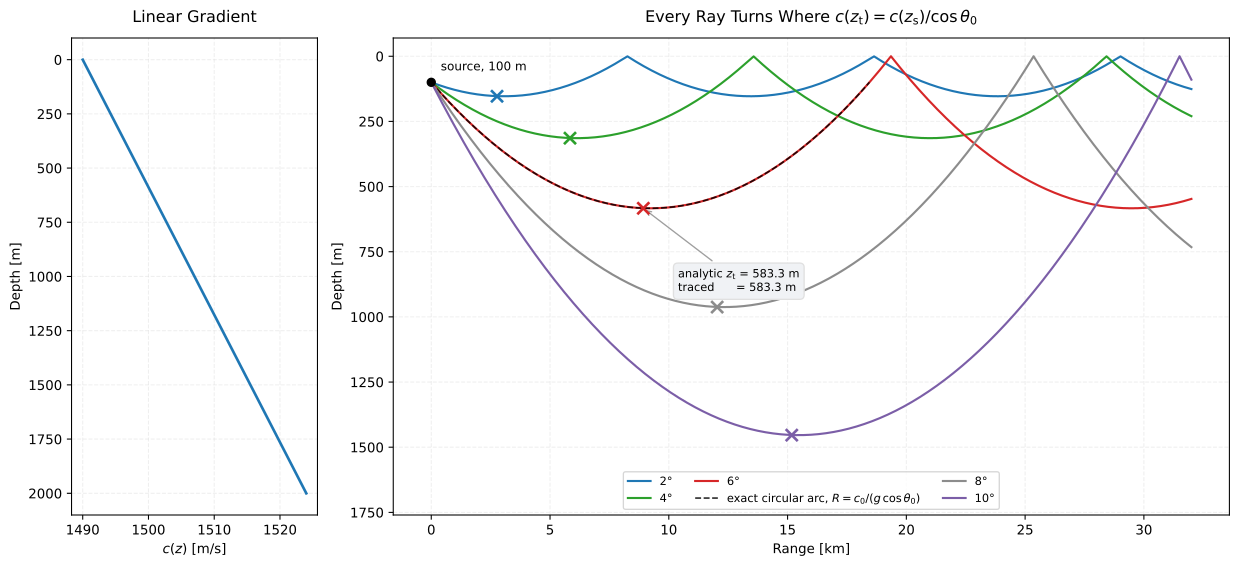

Steeper launch means deeper turn: in the same water the 2° ray turns at 154 m and the 10° ray at 1454 m. The 6° ray carries the page’s own validation, the 583.3 m analytic turning depth, which the trace reproduces to the tenth of a metre it prints, and the dashed overlay is the exact circular arc of radius $R=c_0/(g\cos {\theta }_0)$ the solver is checked against. A result draws its own fan with rays.plot().

import matplotlib.pyplot as plt
import numpy as np

c_top, grad, z_source = 1490.0, 0.017, 100.0
c_source = c_top + grad * z_source
fig, (ax_c, ax_r) = plt.subplots(1, 2, figsize=(13, 6),
                                 gridspec_kw={"width_ratios": [1, 3.4]})
zz = np.linspace(0.0, 2000.0, 200)
ax_c.plot(c_top + grad * zz, zz)
ax_c.invert_yaxis()
ax_c.set(xlabel="c(z) [m/s]", ylabel="Depth [m]")

for angle in (2.0, 4.0, 6.0, 8.0, 10.0):
    rays = underwater.ray_trace([0.0, 2000.0], [c_top, c_top + grad * 2000.0],
                                source_depth=z_source,
                                launch_angles_deg=[angle], max_range=32e3,
                                n_steps=20000)
    ax_r.plot(rays.ranges[0] / 1000.0, rays.depths[0], label=f"{angle:.0f} deg")
    z_turn = (c_source / np.cos(np.radians(angle)) - c_top) / grad
    print(f"{angle:4.0f} deg -> analytic {z_turn:7.1f} m, "
          f"traced {float(rays.depths.max()):7.1f} m")
ax_r.set_ylim(1760.0, -70.0)
ax_r.set(xlabel="Range [km]", ylabel="Depth [m]")
ax_r.legend()
plt.show()

Rays buy geometry and timing: paths, turning depths, convergence-zone ranges and the travel time along every one of them, at a cost independent of frequency. Because the time rides the same four Runge-Kutta stages as the trajectory, and takes its sound speed from the interpolation those stages already do, it describes the path actually returned rather than a second reading of it, and it matches the closed form for a constant gradient (Medwin & Clay 1998, Eq. (3.3.20)) to about $10^{-14}$ s. RayTraceResult still reports no level of its own: the classical per-path amplitude belongs to the eigenrays below, which are the paths a given receiver actually collects, and a field that stays finite where the classical amplitude diverges is section 4’s, on the same rays and through the same marcher.

Passing a bathymetry pair of node arrays, (ranges_m, depths_m), replaces the level bottom with a piecewise-linear depth profile — the faceted boundary of Jensen Fig. 3.20 — while the sound-speed profile stays range independent. The marcher finds each crossing against the interpolated polyline and reflects the ray specularly about the local facet (Eq. 3.121), so a bounce off a slope of angle $\beta$ turns the ray by $2\beta$: upslope bounces steepen a ray, downslope bounces flatten it, and that is the whole one-line physics of wedge propagation. Snell’s invariant is then a constant of each ray only between bottom bounces, and one consequence is faced rather than papered over: a ray steepened past the vertical would run backward in range, which a marcher whose independent variable is range cannot carry, so it is terminated at that bounce and its samples are NaN from there on — a plot simply ends where the ray turned. In an isovelocity wedge every ray is straight lines and mirrors, so every angle below is exact:

import numpy as np
from phonometry import underwater

# An isovelocity wedge: the bottom shoals from 1000 m to 650 m over 4 km, a
# 5 degree upslope. A surface bounce only flips the ray; a bottom bounce
# steepens it by twice the slope.
beta = np.radians(5.0)
wedge = underwater.ray_trace(
    [0.0, 1000.0], [1500.0, 1500.0], source_depth=400.0,
    launch_angles_deg=[20.0], max_range=4000.0, n_steps=1601,
    bathymetry=([0.0, 4000.0], [1000.0, 1000.0 - 4000.0 * np.tan(beta)]))
r, z = wedge.ranges[0], wedge.depths[0]
events = wedge.bottom_reflections[0] + wedge.surface_reflections[0]
incline = np.degrees(np.arctan(np.abs(np.diff(z)) / np.diff(r)))
for leg in range(int(events[-1]) + 1):
    seg = np.flatnonzero(events[:-1] == leg)[1:-1]
    print(leg, round(float(np.median(incline[seg])), 1))
# 0 20.0   as launched
# 1 30.0   first bottom bounce: steepened by 2 beta
# 2 30.0   the surface only flips the sign
# 3 40.0   second bottom bounce: 2 beta again

The polyline starts at $r=0$, so the water column at the source is stated rather than extrapolated, and it continues level past its last node, the same clamp the sound-speed profile lives by; a vertex reflects specularly off one of its two facets, and a bathymetric feature narrower than one range step can hide between two samples of the crossing search, so n_steps has to resolve the bathymetry as well as the rays. eigenrays declines a sloping trace, and says why: each slope bounce rotates Snell’s invariant, so an arrival’s bottom touches no longer share one grazing angle and the one-coefficient-per-path amplitude convention below stops holding.

The fan draws every path the profile supports; a receiver is reached by only a few of them. Those are the eigenrays, “the rays which pass through that point” (Jensen §3.3.5.2), and their list — a delay, a launch and an arrival angle, the boundary-touch counts and a complex amplitude per path — is the arrival structure the sonar equation consumes as multipath, the skeleton of a channel impulse response, and what communications work equalises against. eigenrays takes the traced fan and one receiver and finds them as roots: an eigenray stands wherever a ray’s depth at the receiver range crosses the receiver depth, so a pair of adjacent fan rays straddling the receiver brackets one, and each bracket is closed by bisection on fresh traces through the same profile, never by interpolating between the traced rays — the two rays of a bracket can carry different bounce histories, and a blend of them is a path the water does not contain (the interpolation hazard of Jensen §3.7.5.1). Every arrival is a real ray, its travel time, angles and bounce counts read off its own trajectory, with the spreading $q$ of the next section riding the same march in its real, point-source form (Eq. 3.63), so the classical amplitude of Eq. (3.65) belongs to the very ray that hit:

# The 100 m isovelocity channel unfolds into mirror images, so every arrival
# is checkable by hand: the n-th one flies straight to an image of the
# receiver, sqrt(r^2 + z_n^2) metres away.
fan = underwater.ray_trace([0.0, 100.0], [1500.0, 1500.0], source_depth=36.0,
                           launch_angles_deg=np.arange(-48.0, 48.5, 0.5),
                           max_range=600.0, n_steps=201)
arr = underwater.eigenrays(fan, receiver_range=500.0, receiver_depth=46.0)
print(arr.travel_times.size)          # 11 arrivals inside the 48 degree fan

# The direct path: 500 m out, 10 m down, no touches, 1/R spreading.
print(round(float(arr.travel_times[0]) * 1e3, 2))       # 333.4 ms
print(round(float(abs(arr.amplitudes[0])) * 500.1, 6))  # 1.0: that is 1/R

# The first echo left the source upward and arrives from above, its sign
# flipped once by the pressure-release surface.
print(int(arr.surface_reflections[1]), int(arr.bottom_reflections[1]))  # 1 0
print(round(float(arr.launch_angles[1]), 2))            # -9.31 degrees: up
arr.plot()   # the impulse-response skeleton: per-path loss against delay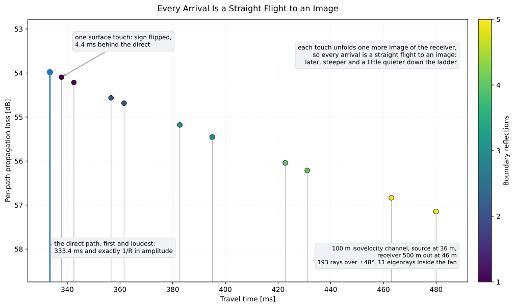

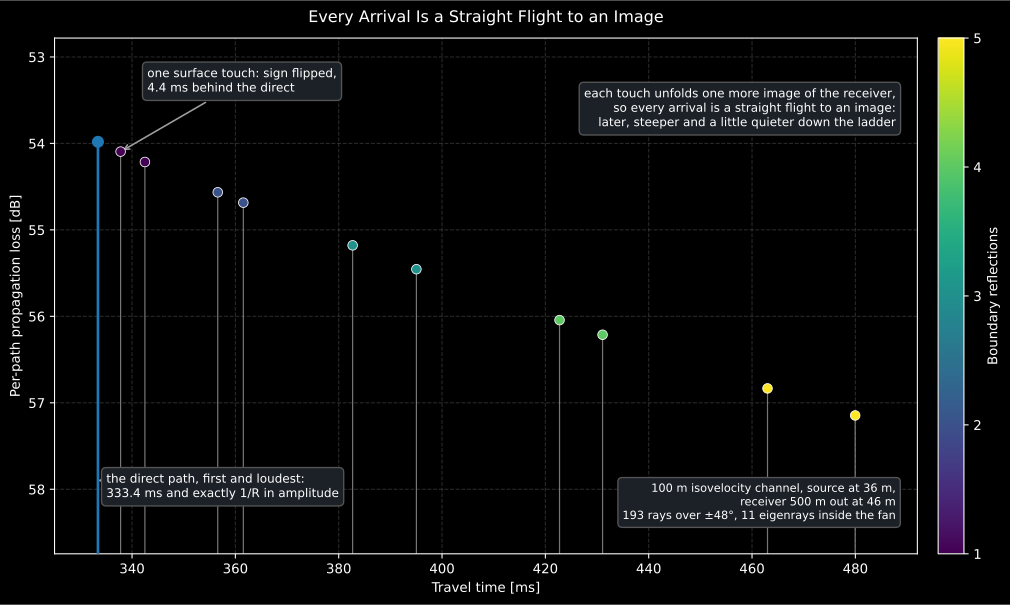
The snippet’s own channel, drawn: one stem per eigenray, its head at that single path’s loss. The direct path arrives first and loudest; the first echo follows 4.4 ms behind, sign flipped by the surface; and each further touch unfolds one more image of the receiver, later, steeper and a little quieter down the ladder. Over perfect reflectors nothing but $1/R$ attenuates a path, so 147 ms of delay spread costs barely 3 dB: this list is the multipath the sonar equation consumes, and the skeleton a channel impulse response is built on.

One list serves every frequency. The amplitudes are normalised to unit pressure at 1 m, in the same $e^{-i\omega t}$ convention as the rest of the module, and the search never asks for a frequency at all: the tone a receiver hears is $p(\omega )={\sum }_j{a}_j{e}^{i\omega {\tau }_j}$, its loss $-20\lg |p(\omega )|$ on the same scale as the other three solvers, and a band’s impulse response is that sum transformed. Each amplitude carries $(-1)$ per surface touch and the bottom’s coefficient per bottom touch — the perfect reflectors’ $\mp 1$, or, with the same FluidSeabed the beams take, the Rayleigh $\mathcal{R}$ of each ray’s own grazing angle, magnitude and phase — and the $(-i{)}^m$ of Eq. (3.79) for each caustic crossed, the discrete form of the $-\pi /2$ the beam solver’s square-root branch spends continuously. Validated against the one environment whose arrival structure is entirely closed form, the ideal waveguide’s image lattice: the count matches image for image, and times, angles and amplitudes agree to $10^{-13}$ s, $10^{-11}$ degrees and $10^{-13}$ relative; and against the $n^2$-linear profile’s exact parabolic ray (Eq. 3.195), whose closed-form travel time, integrated by quadrature to machine precision, the upward-refracted eigenray reproduces to $2\times 10^{-7}$ s, the residual being the sampled profile rather than the search.

Three limits, all deliberate. The fan is the search space: an eigenray steeper than the traced aperture does not exist to it, and a pair of arrivals standing between the same two fan rays merges into no bracket at all, so the fan’s density and half-angle are the completeness levers, and they stay where they are visible, in the ray_trace call. The multipath ladder of a hard-bottomed guide is unbounded, so max_arrivals (64 by default) keeps the earliest arrivals, the flat, least-bounced ones that carry the energy, and warns when it truncates. And the amplitude is classical on purpose: a receiver standing exactly on a caustic is answered with the infinity Eq. (3.65) really has there, because a list of discrete paths is ray theory and says so; the field that stays finite on that caustic is the next section’s, built by widening these same rays into beams.

Section 3 stops at geometry on purpose. The classical ray amplitude (Jensen Eq. 3.65) divides by the ray-tube spreading $q$, and $q$ vanishes wherever the family of rays folds over on itself. That fold is a caustic: ray theory answers infinity there while the true field is merely loud, and a ray that crosses one picks up a $-\pi /2$ that the whole interference pattern beyond it depends on (Jensen §3.4.1, Figs. 3.13-3.14). Past the last ray of a family lies a shadow zone, where ray theory returns not a small number but no number at all.

Gaussian beam tracing removes both at once, by widening every ray into a beam. The spreading obeys the dynamic ray equations (Jensen Eq. 3.58),

which the ray marcher integrates alongside the trajectory. Started from complex initial conditions, $p(0)=1$ and $q(0)=i\omega W_0^2/2$ (Eq. 3.91), each ray becomes the axis of a beam of initial half-width $W_0$ and flat wavefront, and the field of that beam is (Eq. 3.88)

with $n$ the distance from the central ray and $\tau$ the travel time along it. The total field is that expression summed over the launch fan with the weights of Eq. (3.92).

Why it stays finite. Eq. (3.58) is linear with real coefficients, so the real and imaginary parts of $(q,p)$ are two real solutions of it, and their Wronskian $q_R{p}_I-q_I{p}_R$ is conserved. The impulses the spreading takes at a profile kink and at a reflection are shears of unit determinant, so they cannot change it either. It starts at $-\omega W_0^2/2$ and stays there, and that single constant carries the whole method: $q$ can never reach zero, so there is no caustic singularity left to patch, no KMAH index to count and no minimum-width floor to impose; $\mathrm{Im}[p/q]<0$ always, so the beam always decays away from its axis; and the beam half-width of Eq. (3.89) collapses to $W(s)=2|q(s)|/(\omega W_0)$, a hyperbola in free space with its waist at the source and the Rayleigh range $k{W}_0^2/2$ for its scale.

import numpy as np
from phonometry import underwater

# Jensen's n^2-linear profile, c(z) = c0/sqrt(1 + 2.4 z/c0) (Eq. 3.77). With
# the source near the bottom the up-going rays turn, their envelope is a
# caustic, and above it the fan runs out into a shadow zone.
c_bottom_ref = 1550.0
z_beam = np.linspace(0.0, 1000.0, 201)
c_beam = c_bottom_ref / np.sqrt(1.0 + 2.4 * z_beam / c_bottom_ref)

beams = underwater.gaussian_beams(600.0, z_beam, c_beam, source_depth=992.5,
                                  max_range=2500.0, range_step=25.0,
                                  fan=underwater.BeamFan(max_angle_deg=45.0),
                                  n_depth_points=80)
print(beams.propagation_loss.shape)            # (80, 101)  depth x range
print(beams.launch_angles.size)                # 439 beams over +-45 degrees
print(round(float(beams.initial_beam_widths[0]), 1))  # 35.9 m: W0, Eq. (3.86)
beams.plot()   # the PL field, on the same frame as parabolic_equation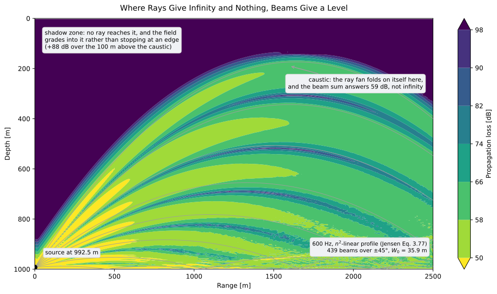

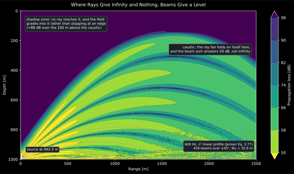
The snippet’s own water, on a finer grid: 600 Hz over the $n^2$-linear profile, the source 7.5 m off the bottom, 439 beams over ±45°. The up-going fan turns inside the column, and where it folds on itself the beam sum answers 59 dB, not infinity — that fold is the bright arc across the top of the dome, and it is the caustic. Above the arc no ray arrives at all, and the field does not stop at that edge: it climbs 88 dB over the 100 m above it, which is the graded penumbra the exact solution has and geometric ray theory does not (Jensen Figs. 3.11, 3.17). The thin grey lines are the rays themselves, traced through the same profile by ray_trace; one beam is hung on each. Two things the picture cannot show: the first three beam widths, about 108 m of range, where the far-field weighting of Eq. (3.92) has nothing to converge to, and the 18% of cells that no beam reaches at all, which are exactly infinite and drawn at the quiet end of the scale.

import matplotlib.pyplot as plt
import numpy as np
from phonometry import underwater

c_ref = 1550.0
z_caustic = np.linspace(0.0, 1000.0, 201)
c_caustic = c_ref / np.sqrt(1.0 + 2.4 * z_caustic / c_ref)

caustic = underwater.gaussian_beams(600.0, z_caustic, c_caustic,
                                    source_depth=992.5, max_range=2500.0,
                                    range_step=12.5,
                                    fan=underwater.BeamFan(max_angle_deg=45.0),
                                    n_depth_points=400)
caustic.plot()   # same field; the figure below bands it and draws the rays
plt.show()

The one free parameter. $W_0$ is it, and the book is candid that “the optimal choice of these initial conditions is a matter of current research”, recommending 10 to 50 wavelengths. The default here is sharper than a rule of thumb, and it is one width per launch angle rather than one per run. In open water §3.5.1 does the optimisation explicitly: differentiating the free-space width of Eq. (3.86) with respect to the complex offset gives $W_0=\sqrt{\lambda r_{\max }/\pi }$, the width that resolves the field best at the far end of the run, where it is resolved worst. That is also where the launch-angle integral behind Eq. (3.92) is a genuine Gaussian rather than a Fresnel integral, which is why it is not merely a tidy choice: against the free field at 100 Hz at 2, 5 and 8 km the error in $|p|$ is $7.5\times 10^{-5}$ at that width, $2.7\times 10^{-2}$ at a fifth of it and $4.1\times 10^{-2}$ at fifteen times it. A shallow channel then raises its own demand on top: its trapped field is a discrete set of modes standing $\lambda /(2D)$ apart in the sine of the launch angle, and a beam mixes launch angles over its far-field divergence $\lambda /(\pi W_0)$, so resolving neighbouring modes to half their gap takes $W_0\ge 4D\cos {\theta }_0/\pi$: one width per launch angle, widest for the flat beams whose modes crowd together, relaxing by the cosine for the steep ones, every beam’s vertical footprint the same $4D/\pi$. The default takes whichever of the two is larger, inside the book’s 10-50 wavelength band, and hands the whole fan the free-space optimum when the channel is too deep in wavelengths for the guide width to fit the band. An earlier version instead capped $W_0$ at a quarter of the water depth, reading the book’s “not large compared to the water depth” as a ceiling on the width rather than on the footprint; what that cap was said to protect, the bookkeeping that folds a reflected ray back into the column, the receiver image ladder already restores, and in shallow water it silently cost decibels of level, always toward too quiet. The measurements are two paragraphs down, cap against default on the same exact oracles.

What it is validated against. Free-field spherical spreading, to $10^{-3}$ dB, which is the one comparison that pins the amplitude normalisation and the phase convention together; the two-ray Lloyd-mirror field with one surface reflection, to 0.01 dB; and the image-source sum of the ideal pressure-release waveguide, to 0.0004 dB with the fan opened to 88 degrees. Over a lossy seabed the same lattice carries $\mathcal{R}(\theta {)}^n$ at each image’s own closed-form angle, and the beams track it to 0.07 dB at worst across both sides of the critical angle. That same guide expanded over its modes instead of its images (Eq. 5.13) is a second closed form of one exact field, and it agrees to 0.03 dB and $8\times 10^{-4}$ rad: it is the comparison that reaches the absolute phase, and it puts the beams on the footing normal_modes and parabolic_equation are already held to. The last one bends the rays, which none of the others do, since $c^{\prime \prime }$ vanishes in an isovelocity channel and takes the coupling coefficient of the dynamic ray equations with it: the $n^2$-linear profile of Eq. (3.77) has exactly linear $k^2(z)$, so its modes are Airy functions with closed-form eigenvalues, and the beams, at their default per-angle width, track them to +0.19 dB in the mean in 200 m of water at 200 Hz and to +0.39 dB in a second, independent 100 m guide at 250 Hz. Those two cuts are also the measurement that retired the old quarter-depth width cap, which on the very same oracles came out +3.08 and +4.12 dB too quiet. Both boundary conditions come out of the beam sum rather than being imposed: the field at a pressure-release surface or bottom is 3 parts in $10^5$ of its mid-column value, and a rigid bottom doubles it.

The water’s own absorption is off by default, so every number above was measured without it and stays reproducible as printed; the price is that the level beyond a few kilometres at sonar frequencies is optimistic. Passing absorption ("francois-garrison", "ainslie-mccolm" or "thorp", or a VolumeAbsorption naming its own water; the same names, arguments and defaults as seawater_absorption) multiplies each beam by $e^{-\alpha s}$ with $s$ the arc length along its central ray, which is Jensen §3.6.2 as printed: perturbing the eikonal with the complex sound speed a volume loss implies leaves the real rays standing and attaches $e^{-{\int }_0^s\alpha d{s}^{\prime }}$ to each (Eq. 3.116). It is not $\alpha r$ over the horizontal range, the shortcut the same section notes “is used in many ray models”: a path at 60° is twice as long as the range it covers, and the steep multiple bounces of a waveguide are exactly the arrivals absorption is supposed to be draining. The marcher integrates $s$ with the same Runge-Kutta stages that place the ray ($ds/dr=1/(\xi c)$), ray_trace exposes it per ray as arc_lengths, and the coefficient, one $\alpha$ per run evaluated at the source frequency and depth, is recorded on the result as absorption_coefficient.

A lossy seabed is the other loss the default leaves out, and in shallow water the dominant one: a perfect bottom hands every steep multiple back undiminished, when what the seabed keeps is most of what decides real shallow-water propagation loss. Passing a FluidSeabed as the bottom (the same fluid description seabed_reflection takes, with water_density for the water above it) replaces the perfect reflector with the Rayleigh coefficient at each beam’s own grazing angle: every bottom touch multiplies the beam’s complex amplitude by $\mathcal{R}$, magnitude and phase together (Jensen §3.6.3, Eqs. 3.125-3.126). The phase is not a refinement to skip: below the critical angle $|\mathcal{R}|=1$ and only the phase distinguishes the lossy seabed from a perfect one, and it moves the interference fringes of every bottom-interacting path. The angle a beam is charged at is the one Snell’s invariant fixes at the bottom, $\cos \theta =\xi c(D)$, the same at every touch of that beam whatever the profile above did in between, so its coefficient is evaluated once, exactly, and raised to the marcher’s count of bottom touches; ray_trace exposes those counts per boundary next to its arc lengths, which is all an amplitude needs of the geometry. Validated against the image lattice with $\mathcal{R}(\theta {)}^n$ at each image’s own closed-form angle: 0.07 dB at worst across ranges whose dominant images sit above and below the critical angle, where stripping the phase from the oracle moves it by 5.7 dB.

The bottom may slope here too: the same bathymetry pair ray_trace takes (section 3) puts every beam’s central ray on the faceted boundary, and the dynamic pair crosses each sloping bounce with the reflection impulse of Eqs. (3.122)-(3.123) evaluated on the local facet. Two of the flat guide’s devices generalise with it, each with its cost stated. The receiver-image ladder folds each receiver column about its own facet — depth and tilt, since a fold plane wrong by the facet’s tilt displaces a first-fold image by metres against a wavelength — so the vertical stack of mirrors becomes the dihedral fan about the local apex, exact for a single facet; at slope zero it is the level ladder bit for bit, which a test pins. And the fan’s wrapped rungs let the beams’ analytic tails carry the arrivals no marched axis can: a path that went up the slope, steepened past the vertical and came back is a wrapped rung, analytic rather than marched. The beam itself, once steepened past the vertical, is terminated at that bounce with its weight zeroed — a range-marching sum keeps only what still travels forward, exactly as the one-way parabolic equation keeps no backscatter — and a tail is trusted no farther than two marched extents from its sample, because beyond that it would be pricing wedge geometry the polyline never described (measured: up to 11 dB of invented field on a tilted bottom no beam can even reach, 0.001 dB with the budget in place). Validated against the ideal wedge, which has an exact solution by images — a fan of $2\pi /\beta$ signed image sources on a circle about the apex, built in the test from pure geometry and proved against both boundary conditions before it judges: a single facet bounce to 0.05 dB, and within 1.85 dB worst / 0.67 dB mean of the complete field across a thin 2.8° wedge whose every cell is dense multipath, most of it arrivals near their own turning point, numbers that move in the fourth decimal when the range step is halved. The lossy fluid seabed above cannot be combined with a slope — one grazing angle per beam is a level-bottom fact, and the solver refuses to pretend otherwise — so a sloping run takes the perfect reflectors of bottom.

Where it stops. Four limits, in the order they bite.

• There is no near field, and this is the biggest error of the four. Eq. (3.92) weights the fan by matching it to a point source in the far field, and Eq. (3.88) divides by a cylindrical range that goes to zero on the axis every ray leaves from, so close in the sum has nothing to converge to. The scale it recovers on is $W_0$, not a fixed distance: over three settings whose $W_0$ spans 150 to 437 m, the worst error against $20\lg R$ in an unbounded medium is 17, 13 and 4.1 dB at a quarter of $W_0$, around 0.6 dB at $W_0$, a hundredth of a decibel at $2.5W_0$ and a thousandth from $3W_0$ out. Read nothing inside about three beam widths of the source, and note that since the default’s free-space width grows as $\sqrt{r_{\max }}$, a longer run pushes that boundary further out. Use parabolic_equation close in.
• Ray theory’s own regime (Jensen §3.4.2): “the wavelength should be substantially smaller than any physical scale in the problem”. This is the limit that bites hardest and that a plausible-looking answer hides best, and an earlier version of this bullet blamed it for an error that was really the width cap’s: at 20 Hz in 100 m of water, where the depth is 1.3 wavelengths and two modes propagate, the capped beam was a third of a wavelength across and the loss came out decibels high against the image-source sum. With the cap retired the same guide measures within 0.03 dB of that sum at the default width. The clean bill is narrower than it looks: an isovelocity column over perfect reflectors is pure geometry, which the folded receiver images reproduce exactly at any frequency, so it says nothing about a channel the low-frequency field actually refracts through. There, normal_modes remains the solver to trust, exact for the cost of a handful of modes.
• The fan is truncated at the fan’s max_angle_deg, and a waveguide with two perfectly reflecting boundaries is the worst case for that, because nothing but $1/R$ attenuates the steep multiple bounces. On the ideal 1000 m guide at 300 Hz, against the image-source sum at 2, 5 and 10 km: 0.27, 4.06 and 2.52 dB with the default 80 degrees, falling to 0.0002, 0.0003 and 0.0004 dB when the fan is opened to 88 degrees. Cutting the oracle to the same half-angle moves it by 0.25, 3.95 and 2.31 dB, so this is the fan and not the method. A real, lossy seabed (the FluidSeabed above) absorbs those bounces and the default is then ample. Opening the fan means cutting range_step with it, since one step has to resolve $\tan {\theta }_{\max }$ depth units of climb per unit range; the solver warns when that pairing is wrong.
• The far shadow is floored. Each beam is summed out to four half-widths, 140 dB below its own axis, so a receiver that no beam of the fan comes that close to gets exactly zero and an infinite loss. That is the unilluminated wedge outside the traced aperture, not the graded penumbra just past the limiting ray, which is where the interesting part of a shadow zone is and which the beams do resolve.

The other flavour, geometric beams (Jensen §3.3.5.5, Eqs. 3.72-3.76), is not implemented. It keeps $q$ real and takes the width from the ray tube itself, $W(s)=|q(s)\delta {\theta }_0|$, so the width vanishes at a caustic and has to be propped up with the Weinberg-Keenan $\pi \lambda$ floor and the KMAH index of Eq. (3.79). That is the patched approach this deliberately does not take, and the book’s own verdict is worth quoting anyway: geometric beams “have generally proven to be more satisfactory” at low frequency, where the physics makes the beam large compared to the channel.

The parabolic equation trades the boundary-value Helmholtz problem for an initial-value problem in range. Factor out the fast outgoing oscillation, $p(r,z)\simeq \psi (r,z)e^{i{k}_{0}r}/\sqrt{k_{0}r}$ with a reference wavenumber $k_0=\omega /c_0$, and for energy travelling within a small angle of the horizontal the envelope obeys the standard (Tappert) PE (Jensen §6.2):

The split-step Fourier algorithm marches it by operator splitting, alternating two individually exact half-physics steps: diffraction is a multiplication by $e^{-i{k}_z^2\Delta r/2k_0}$ in the vertical-wavenumber domain, and refraction a phase screen $e^{i{k}_0(n^2-1)\Delta r/2}$ back in depth, with one transform pair per range step. parabolic_equation starts from a Gaussian field matched to the point source and uses a discrete sine transform in depth, which enforces the pressure-release surface and bottom by construction. The price is the paraxial approximation: the standard PE is accurate within roughly ±15-20° of the horizontal, and steeper energy carries a phase error that shows at short range in shallow waveguides (Jensen §6.2). The free-field calibration is the oracle: with no gradient at all, the marched field must reproduce spherical spreading,

import numpy as np
from phonometry import underwater

# Free field: in a 5000 m isovelocity column, before any boundary is felt,
# the PE must reproduce spherical spreading, PL = 20 lg R.
field = underwater.parabolic_equation(50.0, [0.0, 5000.0], [1500.0, 1500.0],
                                      source_depth=2500.0, max_range=2000.0,
                                      range_step=10.0)
iz = np.argmin(np.abs(field.depths - 2500.0))
ir = np.argmin(np.abs(field.ranges - 1000.0))
print(round(float(field.propagation_loss[iz, ir]), 2))   # 60.0 = 20 lg 1000

and it does so to about $10^{-4}$ dB at the default range step. That is the check the PE cannot fail: free field, no boundaries, no steep energy. The paraxial limit is only visible where those three are absent.

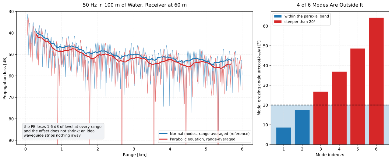
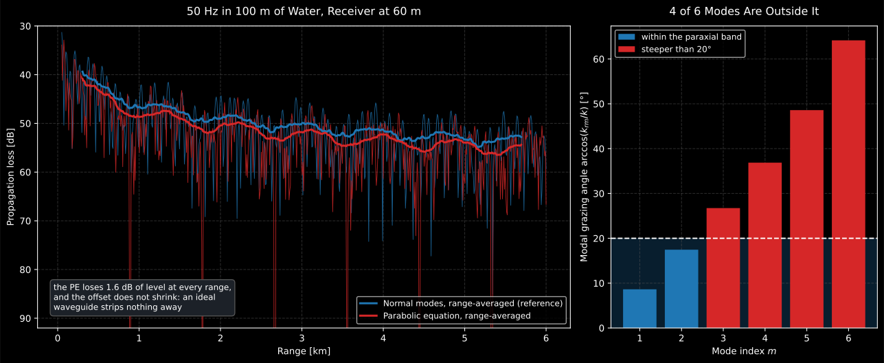
In a 100 m waveguide at 50 Hz, four of the six propagating modes leave the source at 27°, 37°, 49° and 64° — outside the band the standard PE is written for. The consequence is on the left: the range-averaged PE loss sits 1.6 dB above the modal reference, at 300 m and still at 5.7 km. The offset does not wash out with range, because an ideal waveguide is lossless and strips nothing away; in a real seabed the steep modes attenuate first and the gap does close. This is the failure mode to look for in your own output — a level that is uniformly a little too low, not a wrong shape.

import matplotlib.pyplot as plt
import numpy as np

r = np.linspace(50.0, 6000.0, 700)
modes = underwater.normal_modes(50.0, [0.0, 100.0], [1500.0, 1500.0],
                                source_depth=30.0, receiver_depth=60.0,
                                ranges_m=r, n_depth_points=800)
pe_field = underwater.parabolic_equation(50.0, [0.0, 100.0], [1500.0, 1500.0],
                                         source_depth=30.0, max_range=6000.0,
                                         range_step=5.0, n_depth_points=1024)
iz2 = int(np.argmin(np.abs(pe_field.depths - 60.0)))
pe_pl = np.interp(r, pe_field.ranges, pe_field.propagation_loss[iz2])

def range_average(pl, width=61):        # incoherent, in the energy domain
    return -10.0 * np.log10(np.convolve(10.0 ** (-pl / 10.0),
                                        np.ones(width) / width, mode="same"))

inner = (r > 300.0) & (r < 5700.0)
sm_nm = range_average(np.asarray(modes.propagation_loss))
sm_pe = range_average(pe_pl)
print(round(float(np.mean(sm_pe[inner] - sm_nm[inner])), 2))   # 1.64 dB

fig, (ax_pl, ax_ang) = plt.subplots(1, 2, figsize=(13.5, 5.6),
                                    gridspec_kw={"width_ratios": [2, 1]})
ax_pl.plot(r / 1000.0, modes.propagation_loss, alpha=0.35)
ax_pl.plot(r / 1000.0, pe_pl, alpha=0.35)
ax_pl.plot(r[inner] / 1000.0, sm_nm[inner], label="Normal modes, averaged")
ax_pl.plot(r[inner] / 1000.0, sm_pe[inner], label="PE, averaged")
ax_pl.set_ylim(30.0, 92.0)
ax_pl.invert_yaxis()
ax_pl.set(xlabel="Range [km]", ylabel="Propagation loss [dB]")
ax_pl.legend()

k0 = 2.0 * np.pi * 50.0 / 1500.0
grazing = np.degrees(np.arccos(np.clip(modes.wavenumbers / k0, -1.0, 1.0)))
ax_ang.bar(np.arange(1, grazing.size + 1), grazing)
ax_ang.axhline(20.0, linestyle="--")
ax_ang.set(xlabel="Mode index m", ylabel="Grazing angle arccos(k_rm/k) [deg]")
plt.show()

The four solvers are configured by the caller, and every snippet above sets a grid without saying why. The rules are short.

The depth grid. The sine transform of the PE, and the finite-difference eigenproblem of the modes, both alias a spectrum that is steep in depth, so the grid is sized in wavelengths. At 50 Hz, $\lambda =30$ m, and a grid near $\lambda /10$ over 5000 m of water means a few thousand interior points — which is why the section 1 snippet’s n_depth_points=512 is labelled the coarse, fast setting rather than the right one. Refine and re-run before trusting a number.

The split-step range step. The refraction half-step is a phase screen $e^{i{k}_0(n^2-1)\Delta r/2}$, so it should turn the phase by well under a radian per step, and be tightened wherever the profile has strong gradients. The honest test is the same one: halve $\Delta r$ and see whether the field moves.

When normal_modes warns. The warning says a retained mode sits inside the finite-difference error band. The remedy is to raise n_depth_points: the eigenvalue error is $O(\Delta z^2)$, and near-cutoff modes are its first casualties — which are exactly the shallow-angle modes that carry the field to long range, so ignoring the warning quietly costs the answer at the ranges you care about.

The ray fan and the ray step. The launch angles are not a free choice either: pick them from Snell’s turning condition so the fan spans the rays the channel traps, rather than the round $\pm 12°$ of the snippet above. The number of steps has to keep the arc length per step small against the vertical scale of the profile, or a turning point is stepped straight over.

The beam fan and the beam width. gaussian_beams takes that same fan and adds two knobs to it. n_beams decides whether neighbouring beams still overlap where they have spread most: adjacent beams are $s\delta {\theta }_0$ apart at arc length $s$ while each has spread to $s\lambda /(\pi W_0)$, so the overlap condition $\delta {\theta }_0\lesssim \lambda /(\pi W_0)$ is range-independent and the default takes four times that margin. Too coarse a fan does not read as a wrong level but as a periodic ripple in range at the beam spacing, which is easy to mistake for physical interference. beam_width is the $W_0$ of section 4, whose default is the optimum only where the channel does not clamp it, so pass it explicitly in shallow water. The three travel together as the BeamFan the solver takes. And opening max_angle_deg means cutting range_step with it, since one step has to resolve $\tan {\theta }_{\max }$ depth units of climb per unit range.

The convergence discipline. Refine, re-run, compare; only then compare solvers. Agreement between the modes and the PE, which section 6 calls the practical convergence test, is worth nothing if neither of them has converged on its own grid.

Every propagation function of the underwater module answers the same question, “how much level survives the path”, at a different price in physics. Terminology throughout follows ISO 18405:2017 (propagation loss, source level, levels re 1 µPa). The sound-speed and absorption models named below are implemented and referenced in Underwater sound propagation.

Sound speed. The four equations agree to within about 1 m/s inside the domain they share — 0.98 m/s at 25 °C, 35 ppt and 1000 m, and 0.52 m/s over the upper kilometre of a full profile, as the model comparison on the propagation page shows — so the choice is about validity range, not accuracy. The default UNESCO / Chen-Millero form (as recast by Wong & Zhu 1995) covers 0–40 °C, 0–40 ppt and 0–1000 bar, the widest envelope, and is the international standard. Del Grosso (1974) is restricted to 0–30 °C and 30–40 ppt but is preferred by some authors for deep-ocean work inside that domain (much of the SOFAR-channel literature uses it). Mackenzie (1981) trades pressure for depth directly (2–30 °C, 25–40 ppt, 0–8000 m), which makes it the convenient choice when you have an echo-sounder depth rather than a CTD pressure; the other two convert depth to pressure through Leroy & Parthiot (1998) internally. Medwin (1975) is a six-term simplification valid to about 1000 m in shallow, warm water; it is the coarsest of the four and the one behind the rules of thumb $\partial c/\partial T\approx 4.6-0.110T$ m/s per °C and $\partial c/\partial z\approx 0.016$ m/s per metre, so keep it for mental arithmetic and hand checks, not for a budget.

Absorption. Francois–Garrison (1982) is the reference and the default: it carries the boric-acid, magnesium-sulfate and pure-water relaxations with their full temperature, salinity, depth and pH-implicit dependences, and is trusted from about 100 Hz to 1 MHz. Ainslie–McColm (1998) is a deliberate simplification of the same physics that stays within about 10 % of it across that range; use it when a legible formula matters more than the last percent. Thorp (1967) depends on frequency only (it bakes in 4 °C water near 1000 m) and predates both; keep it for quick low-frequency estimates below a few tens of kHz and for comparison with older literature that used it.

Spreading law. Spherical spreading ($20{\log }_{10}R$) describes a wavefront that expands freely in three dimensions, before any boundary confines it; cylindrical spreading ($10{\log }_{10}R$) describes energy trapped between the surface and the bottom (or in the SOFAR channel) that can only expand in range. The "practical" law splices the two at a transition range $R_0$, which is physically of the order of the water (or channel) depth: spherical while the wavefront has not yet filled the duct, cylindrical once it has. In the 10 kHz example of the propagation-loss section the choice is not cosmetic: against the same figure of merit of 87 dB, spherical-only spreading predicts detection out to about 8.7 km while the practical law with $R_0=1000$ m stretches it to about 15.8 km. When the spreading law is the biggest uncertainty in the budget, that is the cue to stop using a closed form and compute the field.

Closed form or solver. The closed-form propagation loss knows nothing of the sound-speed profile, the seabed or the surface; it is honest for short, direct, boundary-free paths and for first-cut sonar budgets. When refraction and boundaries decide the answer, pick the solver by frequency and geometry (Jensen et al. 2011, Ch. 1):

The boundaries blur in practice: rays remain usable at surprisingly low frequencies for travel-time work, and the PE remains the workhorse well above its formal small-angle regime. When two of the four agree on a case, as the modes and the PE do in the section 1 figure, that agreement is the practical convergence test. The two extremes divide the labour cleanly: normal_modes and parabolic_equation both get more expensive as the frequency rises, since both have to resolve the wavelength on a grid, while the ray core does not, so gaussian_beams is the one that stays affordable exactly where the others stop being so, and it is also the one whose approximation is best justified there.

Chain the pieces end to end: a 140 dB re 1 µPa²/Hz source at 10 kHz, a 60 dB ambient spectrum level, a 15 dB array gain and an 8 dB detection threshold give the figure of merit $FOM=140-(60-15)-8=87$ dB, computed by passive_sonar_equation in the sonar-equation section of the propagation guide. Every term then moves the crossing of the propagation-loss curve of that guide’s propagation-loss section (10 °C, 35 ppt, 100 m), and that crossing is the predicted detection range.

import numpy as np

env = {"temperature": 10.0, "salinity": 35.0, "depth": 100.0}
se = underwater.passive_sonar_equation(
    source_level=140.0, propagation_loss=np.linspace(40.0, 120.0, 400),
    noise_level=60.0, directivity_index=15.0, detection_threshold=8.0)
print(se.figure_of_merit)                                    # 87.0 dB

for law, r0 in (("spherical", None), ("practical", 1000.0)):
    res = underwater.detection_range(se.figure_of_merit, 10e3, law=law,
                                     transition_range=r0, **env)
    print(law, round(float(res.detection_range) / 1000.0, 1))  # 8.7 / 15.8 km

# Two ways to lose it: half the array gain, or double the frequency.
trim = underwater.passive_sonar_equation(
    source_level=140.0, propagation_loss=np.linspace(40.0, 120.0, 400),
    noise_level=60.0, directivity_index=7.5, detection_threshold=8.0)
print(trim.figure_of_merit)                                  # 79.5 dB
print(round(float(underwater.detection_range(
    trim.figure_of_merit, 10e3, law="practical",
    transition_range=1000.0, **env).detection_range) / 1000.0, 1))       # 10.0 km
print(round(float(underwater.detection_range(
    se.figure_of_merit, 20e3, law="practical",
    transition_range=1000.0, **env).detection_range) / 1000.0, 1))       # 5.9 km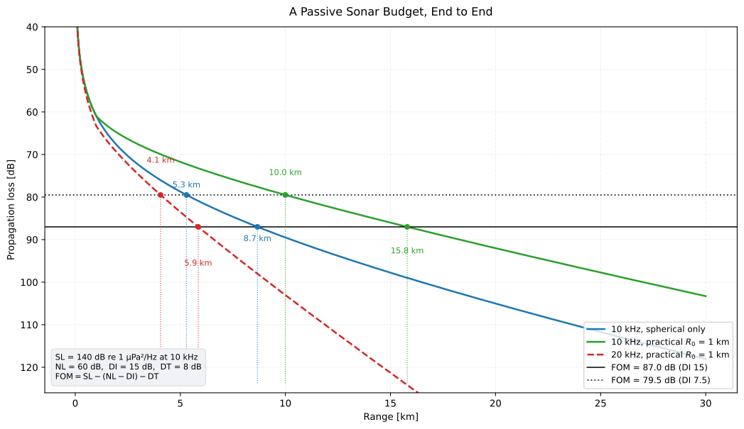

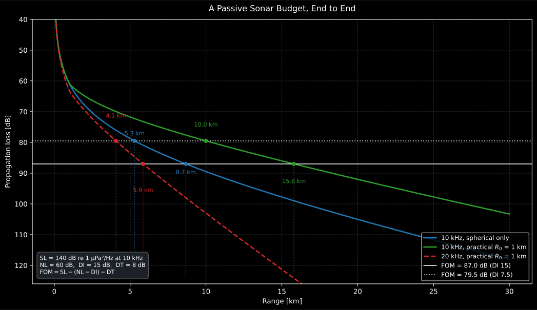
The same source and the same sea, six answers between 4.1 and 15.8 km. The spreading law is the biggest lever: choosing spherical-only over the practical law with $R_0=1$ km costs 7.1 km at 10 kHz. Halving the array gain costs 5.8 km; doubling the frequency costs 9.9 km, because $\alpha$ goes from 0.95 to 3.30 dB/km. When the spreading law is the biggest uncertainty in a budget, that is the cue to stop using a closed form and compute the field.

import matplotlib.pyplot as plt

ranges = np.linspace(50.0, 30_000.0, 800)
fig, ax = plt.subplots(figsize=(11, 6.4))
cases = (("10 kHz, spherical only", 10e3, "spherical", None),
         ("10 kHz, practical R0 = 1 km", 10e3, "practical", 1000.0),
         ("20 kHz, practical R0 = 1 km", 20e3, "practical", 1000.0))
for label, freq, law, r0 in cases:
    ax.plot(ranges / 1000.0,
            underwater.propagation_loss(ranges, freq, law=law,
                                         transition_range=r0, **env).pl,
            label=label)
for fom in (se.figure_of_merit, trim.figure_of_merit):
    ax.axhline(fom, linewidth=1.4, label=f"FOM = {fom:.1f} dB")
    for _label, freq, law, r0 in cases:
        r50 = float(underwater.detection_range(fom, freq, law=law,
                                               transition_range=r0,
                                               **env).detection_range)
        ax.plot([r50 / 1000.0], [fom], "o")
ax.set_ylim(40.0, 126.0)
ax.invert_yaxis()
ax.set(xlabel="Range [km]", ylabel="Propagation loss [dB]")
ax.legend()
plt.show()

One number in that budget deserves a second look. A 60 dB ambient spectrum level at 10 kHz is well above what the sea alone produces: ocean_ambient_noise gives 42 dB re 1 µPa²/Hz there in a 15 knot wind. Sixty decibels therefore describes a noisy site or a self-noise-limited receiver, not a quiet ocean — and noticing that is the difference between a budget and an arithmetic exercise. This coupling between the absorption model, the spreading law and the sonar equation is why they all live in one module.

• Covered

  normal_modes, ray_trace, gaussian_beams and parabolic_equation implement the Jensen et al. (2011) numerical solvers for a range-independent stratified ocean: the finite-difference Sturm-Liouville modal sum (Ch. 5, Eqs. 5.3-5.17), the Runge-Kutta ray-trajectory integration (Ch. 3, Eqs. 3.23-3.24), the Gaussian beam sum built on it (Ch. 3, §3.5, Eqs. 3.88-3.92) and the split-step Fourier standard PE (Ch. 6), with ISO 18405:2017 terminology throughout. ray_trace also returns the travel time along each ray, integrated as a third state of the same Runge-Kutta step, and eigenrays searches a traced fan for the arrivals that join a source to one receiver, each refined by bisection on fresh traces and charged the classical ray amplitude of Eq. (3.65) with the boundary and caustic phases on record (Eqs. 3.79, 3.125-3.126). ray_trace and gaussian_beams also accept a piecewise-linear bottom profile, the faceted boundary of Ch. 3 reflecting each ray about the local facet (Eq. 3.121) with the dynamic pair crossing the bounce by Eqs. (3.122)-(3.123). Each is validated against an exact closed form: the ideal pressure-release waveguide’s modes and its image-source sum (for the eigenrays, that lattice’s complete arrival list, time, angle, count and amplitude per image), the circular-arc rays of a linear gradient together with the published travel time along them (Medwin & Clay 1998, Eq. (3.3.20)), free-field spherical spreading, and, for the sloping bottom, the ideal wedge’s exact closed fan of images, plus the mutual agreement of the modal and PE propagation loss.

• Not covered

  All four solvers assume a range-independent water column with a pressure-release surface, and the bottom is a perfect reflector by default, pressure-release or (for the modes and the beams) rigid. The beams can trade it for the lossy fluid seabed of the Rayleigh model (level bottoms only), and the two ray-based solvers can slope the bottom over a piecewise-linear depth profile, which is the only range dependence there is: a range-dependent water column $c(r,z)$ is excluded deliberately, because the sloping boundary has an exact oracle (the ideal wedge’s closed image fan) and $c(r,z)$ has none. There is no elastic bottom and no sediment attenuation. The ray solver returns paths and travel times, not amplitudes; the per-path level belongs to eigenrays, whose arrival list is classical ray theory and honestly diverges for a receiver standing on a caustic, while gaussian_beams is what supplies a finite field, by summing beams rather than by finding rays. Its geometric-beam alternative (Ch. 3, §3.3.5.5) with the KMAH index and the Weinberg-Keenan width floor is not implemented. The PE is the standard small-angle (Tappert) form, not a wide-angle Padé variant. For the elastic seabed physics these fluid solvers leave out, see Elastic waves and fluid-solid coupling.

Pick by frequency and geometry (Jensen et al. 2011, Ch. 1): rays for high frequency and deep water (ray-path geometry, travel times and convergence zones at a cost independent of frequency, over a level or sloping bottom, plus, through eigenrays, the per-receiver arrival list), Gaussian beams when that same high-frequency geometry has to yield a level (the PL($z$,$r$) field, finite at caustics and graded into shadow zones), normal modes for low frequency in shallow water (few propagating modes, $M\approx kD/\pi$, the reference solution for its regime) and the parabolic equation for low-frequency, long one-way paths (the full PL($z$,$r$) field with refraction). When two solvers agree on a case, that agreement is the practical convergence test.

When refraction or boundaries decide the answer: a sound-speed minimum that traps energy (the SOFAR channel), surface and bottom reflections in shallow water, or a detection range that swings with the choice of spreading law. The closed form $PL=\text{spreading}+\alpha R$ is honest for short, direct, boundary-free paths and first-cut sonar budgets; beyond that, compute the field.

References

Section titled “References”- International Organization for Standardization. (2017). Underwater acoustics — Terminology (ISO 18405:2017). The standardized definitions (propagation loss, source level, sound pressure level re 1 µPa) behind the quantities of this page.
- Jensen, F. B., Kuperman, W. A., Porter, M. B., & Schmidt, H. (2011). Computational ocean acoustics (2nd ed.). Springer. https://doi.org/10.1007/978-1-4419-8678-8The reference monograph implemented here: the modal derivation of section 2 (Ch. 5, Eqs. 5.3-5.17), the ray equations of section 3 (Ch. 3, Eqs. 3.23-3.24) and its eigenray arrivals (§3.3.5, Eqs. 3.65-3.68), the Gaussian beams of section 4 (Ch. 3, §3.5, Eqs. 3.88-3.92), the split-step Fourier parabolic equation of section 5 (Ch. 6) and the model-selection guidance of section 6 (Ch. 1).
- Munk, W. H. (1974). Sound channel in an exponentially stratified ocean, with application to SOFAR. The Journal of the Acoustical Society of America, 55(2), 220-226. https://doi.org/10.1121/1.1914492The canonical deep-water sound-speed profile used by the section 1 figure and snippets.