Underwater acoustics: radiated noise and pile driving

Standards: ISO 18405 ISO 17208 ISO 18406Key references: Urick 1983 Ainslie 2010

Underwater sound is referenced to 1 µPa (not the 20 µPa of airborne acoustics), and its exposure to 1 µPa²·s. This page covers the ISO 18405 reference levels realised as the shared primitives, the ISO 17208 ship radiated noise level and equivalent monopole source level, and the ISO 18406 percussive pile-driving single-strike, peak and cumulative sound exposure. Every quantity is an exact closed form, verified analytically.

1. Reference levels (ISO 18405)

Three primitives, referred to 1 µPa, are computed from a captured pressure signal. Every pressure argument on this page is in pascals — calibrated hydrophone output with no weighting applied — and every level comes out re 1 µPa (or re 1 µPa²·s):

SPL = 10 lo g_{10} \frac{⟨ p ^{2} ⟩}{p _{0}^{2}}, SEL = 10 lo g_{10} \frac{\int p ^{2} d t}{E _{0}}, L_{p, pk} = 20 lo g_{10} \frac{max ∣ p ∣}{p _{0}},

with $p_{0} = 1 μ Pa$ and $E_{0} = 1 μ Pa^{2} s$ . The sound pressure level is the mean-square level (ISO 18406 Formula 7); the sound exposure level integrates the squared pressure over the record (ISO 18406 Formulae 3-4); the peak level is the zero-to-peak value, the greatest magnitude of $p (t)$ over the pulse, of either sign (ISO 18406 Formula 5 with its Note 1).

That convention is worth pinning down before any number is compared against a limit. Much of the pile-driving literature, and several older consent conditions, quote a peak-to-peak level instead, which for a symmetric pulse runs about 6 dB higher; the standard also lets the compressional and rarefactional peaks be reported separately (Clause 8.4.2). A computed peak_sound_pressure_level is zero-to-peak, so establish which convention an external threshold uses before subtracting one from the other.

from phonometry import underwater

spl = underwater.sound_pressure_level(pressure)        # dB re 1 µPa
sel = underwater.sound_exposure_level(pressure, fs)     # dB re 1 µPa²·s
pk = underwater.peak_sound_pressure_level(pressure)     # dB re 1 µPa

To re-reference a level between the underwater (1 µPa) and airborne (20 µPa) conventions (a $20 lo g_{10} (20) \approx 26.02$ dB shift, not an energy/intensity equivalence), use underwater_to_in_air_spl / in_air_to_underwater_spl. For background-noise subtraction, reuse the ISO 3744 background_noise_correction ( $K_{1}$ ) helper.

2. Ship radiated noise and source level (ISO 17208-1/-2)

A surface ship measured in deep water is described first by its radiated noise level and then by an equivalent monopole source level:

L_{RN} = 20 lo g_{10} \frac{p _{rms}}{p _{0}} + 20 lo g_{10} \frac{r}{r _{0}} dB re 1 μ Pa \cdot m, L_{s} = L_{RN} + Δ L,

where the Lloyd’s-mirror surface correction (ISO 17208-2 Formula 3) for a nominal source depth $d_{s} = 0.7 D$ ( $D$ = mean draught) and $u = k d_{s}$ , $k = 2 π f / c$ , is

Δ L = - 10 lo g_{10} \frac{2 u ^{4} + 14 u ^{2}}{14 + 2 u ^{2} + u ^{4}} dB .

The correction exists because of the sea surface. To a receiver below, the surface is a pressure-release mirror, so the ship radiates as a source plus a phase-inverted image a distance $2 d_{s}$ above it — the dipole of ISO 17208-2 Annex A. When the pair is shallow in wavelength terms the two nearly cancel, so the field measured below understates what an equivalent monopole would have to be; when it is deep in wavelength terms the two decorrelate over the measurement aperture and radiate twice the power of one alone.

Read the limits as that statement. $Δ L$ grows without bound as $u \to 0$ (the argument of the logarithm tends to $u^{2}$ ), which is low frequency or small draught: there the conversion is inverting a near-total cancellation, so a small error in the assumed source depth or sound speed becomes a large error in source level, and the low-frequency end of a reported source-level spectrum is the least trustworthy part of it. It crosses zero at $u \approx 1.03$ — 59 Hz for the 4.2 m source depth of the example below — and tends to $- 10 lo g_{10} (2) = - 3.01$ dB as $u \to \infty$ , where source and image add incoherently.

The nominal source depth itself is a convention, not a located source: ISO 17208-2 Formula (1) fixes $d_{s} = 0.7 D$ on the mean of the bow and stern draughts and its own Note 4 calls the choice “somewhat arbitrary”, a compromise. The reported source level is therefore an equivalent monopole broadside value that means nothing on its own — Clause 6.2 requires the nominal source depth, the sound speed used and the conversion formula applied to be reported with it.

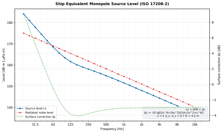
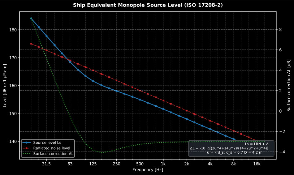
Ship radiated noise level and equivalent monopole source level versus frequency, with the Lloyd's-mirror surface correction on a twin axis showing its low-frequency divergence and its approach to −3 dB at high frequency

The gap between the two curves is the surface correction, and it changes sign. For this 6 m draught ( $d_{s}$ = 4.2 m) it adds 9.08 dB at 20 Hz, crosses zero near 59 Hz, overshoots to −4.07 dB at 160 Hz and only then settles on the $- 10 lo g_{10} (2) = - 3.01$ dB of an incoherent source-plus-image pair, which it reaches by 4 kHz. Everything left of the crossing is the inversion of a near-total cancellation: that is the part of a published source-level spectrum that moves most when the assumed source depth is wrong.

Show the code for this figure

import numpy as np
from phonometry import underwater

freqs = np.array([20, 25, 31.5, 40, 50, 63, 80, 100, 125, 160, 200, 250, 315,
                  400, 500, 630, 800, 1000, 1250, 1600, 2000, 2500, 3150,
                  4000, 5000, 6300, 8000, 10000, 12500, 16000, 20000.0])
rnl = 175.0 - 12.0 * np.log10(freqs / 20.0)
res = underwater.monopole_source_level(rnl, freqs, draught=6.0)
res.plot()

import numpy as np
from phonometry import underwater

# Band r.m.s. pressures measured at 100 m from a merchant ship, in pascals.
freqs = np.array([31.5, 63.0, 125.0, 250.0, 500.0, 1000.0])
p_rms = np.array([4.3, 2.8, 1.9, 1.2, 0.8, 0.54])
rnl = np.array([underwater.radiated_noise_level(float(x), 100.0) for x in p_rms])
print(np.round(rnl, 1))   # [172.7 168.9 165.6 161.6 158.1 154.6] dB re 1 uPa.m

# The surface correction is frequency-dependent, so the conversion is normally
# run on the whole band vector at once.
res = underwater.monopole_source_level(rnl, freqs, draught=6.0)
print(np.round(res.source_level, 1))       # [177.8 168.4 161.7 157.8 154.8 151.6]
print(np.round(res.surface_correction, 2))  # [ 5.15 -0.51 -3.86 -3.78 -3.27 -3.08]
print(round(res.source_depth, 2))           # 4.2 m = 0.7 x draught
res.plot()   # RNL, Ls and ΔL vs frequency (needs matplotlib)

Read the magnitudes before going on. A merchant ship lives at a radiated noise level of roughly 160-180 dB re 1 µPa·m, against ocean ambient spectrum levels of 60-100 dB, so a result far outside that range is a units error rather than a quiet ship. Above the first Lloyd’s-mirror null the correction settles towards $- 3$ dB and the equivalent monopole level sits just below the radiated noise level; only at the lowest bands, where $u$ is small, does it go the other way.

hydrophone_depths gives the three ISO 17208-1 measurement depths from the 15°/30°/45° depression angles, and source_level_uncertainty the tabulated expanded uncertainty (5 dB ≤100 Hz, 3 dB 125 Hz–16 kHz, 4 dB >16 kHz).

Those tabulated figures are the uncertainty of the radiated noise level, and they are representative values rather than a budget for your survey. ISO 17208-2 Clause 5 adds two more terms to the source level. The sound speed enters only through $k d_{s}$ , so even a 10 % error in it costs under a decibel. The fitted correction departs from the full Lloyd’s-mirror expression by less than 2 dB in nearly every decidecade band, with one exception: about 4 dB in the band where $k d_{s} \approx 13$ , which for the 4.2 m source depth of the example above is 739 Hz — worth computing for your own draught before reporting. The third term, the adequacy of describing a directional multi-mechanism radiator as a single monopole, the standard declines to quantify at all and leaves to the user. One validity condition sits underneath all of it: ISO 17208-1 Clause 6.2 requires the signal-plus-noise to noise level difference to be at least 3 dB in a band for that band’s level to count, between 3 dB and 10 dB with the background correction applied and declared, and above 10 dB uncorrected.

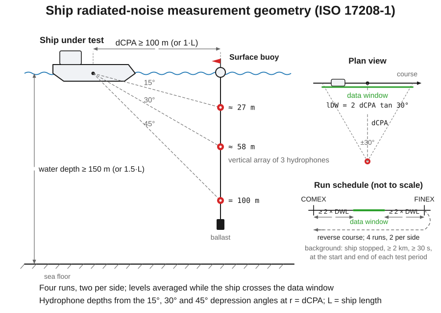
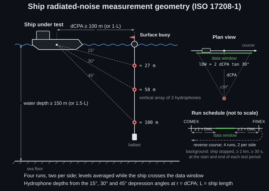
What turns these closed forms into a comparable number is the measurement discipline ISO 17208-1 wraps around them. The ship transits a straight course past a vertical string of three hydrophones at a closest point of approach of 100 m or one ship length, whichever is greater, in water at least 150 m or 1.5 ship lengths deep so the bottom stays out of the picture (Clauses 5.2, 5.4). Only the data window of ±30° about the CPA is scored: the averaging runs while the ship crosses a window of length $2 d_{C P A} tan 30°$ (about 1.15 CPA distances), centred on the beam aspect the radiated noise level is defined for (Clause 3, Figure 3). Four runs are required, two per side; each run’s three hydrophone levels are power-averaged (ISO 17208-1 Formula 8), the runs are then arithmetically averaged (ISO 17208-1 Formula 9), and port and starboard are also reported separately, because a real ship does not radiate symmetrically (Clause 6.5). Background noise is measured at the start and end of each test period and the ISO 3744-style correction applied per band; the recommended wind limit is 20 kn for ships above 100 m (Clause 5.3).

The instrument half is equally prescribed, and it is what the closed forms above assume. Three hydrophones, omnidirectional over 10 Hz to 20 kHz (to 50 kHz if a ship’s noise criteria ask for it), with sensitivity and directivity known to within ±2 dB; all three channels acquired simultaneously and sample-accurately, with the tracking and time-stamp data recorded synchronously so the track can be reconstructed; decidecade processing to IEC 61260 Class 1, with linear frequency-domain averaging over one data-window period (Clauses 4.2, 4.3). Portable hydrophones are laboratory-calibrated to IEC 60565 every 12 months, fixed ones before installation and confirmed every 12 months against a calibrated source or reference hydrophone, and both get an insert-voltage field calibration daily during measurements (Table 1). The geometry has acceptance limits, not just a nominal value: ranging accurate to 10 % of the CPA distance, the actual CPA within −10 % to +25 % of nominal, and the hydrophone cable drift angle under 5° or else reduced or accounted for in the slant range (Clause 4.4). So does the run: COMEX and FINEX at least two data-window lengths either side of the CPA, constant speed, fixed machinery and minimum helm from one to the other, a reverse-course turn between runs, and background measured with the ship stopped at least 2 km away for at least 30 s. If the wind changes by more than 5 kn, or sea state, traffic or precipitation change, the survey is suspended and the background re-measured (Clause 5.6). Finally there is a disposal rule, which is the one most often skipped: bands that stay background-limited after correction are flagged as background-limited or not presented at all (Clause 5.2). Skip any of this and the number you quote is a level, but not an ISO 17208 radiated noise level.

All of that discipline fits in one picture: the transit geometry in section and the data window in plan.

ISO 17208-1 deep-water measurement geometry: a ship transiting past a surface buoy that suspends a vertical array of three hydrophones at depths of about 27, 58 and 100 metres set by the 15, 30 and 45 degree depression angles, a lateral distance at the closest point of approach of at least 100 metres or one ship length, water at least 150 metres deep, and a plan view showing the plus or minus 30 degree data window about the CPA

3. Pile-driving sound (ISO 18406)

Percussive pile driving radiates one impulsive pulse per hammer strike. Each strike has a single-strike sound exposure level $SEL_{ss}$ ; over a driving sequence the exposures add to a cumulative sound exposure level:

SE L_{cum} = 10 lo g_{10} n \sum 1 0^{SEL_{n} /10}, and for N identical strikes = SE L_{ss} + 10 lo g_{10} N .

The energy sum on the left is the definition; the $+ 10 lo g_{10} N$ form on the right is the special case in which every strike is the same, and a real drive is not. A soft start deliberately runs at reduced hammer energy, and the radiated level then grows as the pile embeds and the driving energy rises, so per-strike exposures across a single pile can span several decibels — which is exactly why ISO 18406 Clause 6.2 requires the monitoring station to record the whole sequence, and Clause 8.2 the per-blow hammer energy history including the soft start. Take the loudest strike as representative and the campaign is overestimated; take an early one and it is underestimated, and the error is largest for the long drives where the cumulative criterion binds. So: use cumulative_sel with the measured per-strike series whenever the record exists, keep cumulative_sel_identical for planning estimates, and when it is used, state which strike the single-strike value came from. Both forms also assume the receiver stays where it is, an assumption the marine-mammal exposure guide returns to.

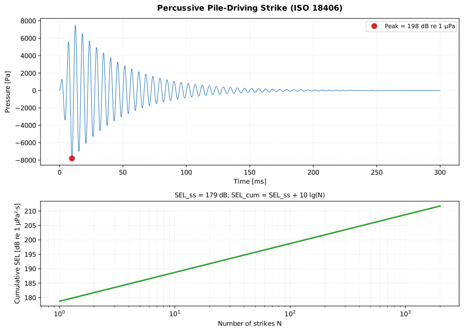
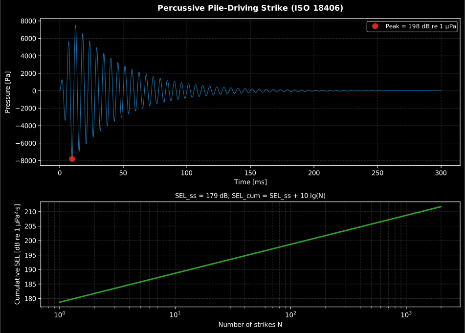
A percussive pile-driving strike pressure waveform with its peak marked, and below it the cumulative sound exposure level growing as SEL_ss plus ten times the logarithm of the number of strikes

The three numbers a single strike yields are not interchangeable, and the figure shows how far apart they sit: this synthetic strike has a peak of 197.9 dB re 1 µPa, a single-strike SEL of 178.7 dB re 1 µPa²·s and a 90 %-energy pulse duration of 60 ms. The lower panel is a straight line on a log-N axis by construction, so a 2000-blow pile adds $10 l g 2000$ = 33.0 dB and reaches 211.7 dB — an injury criterion written on cumulative SEL is met by the count as much as by the hammer.

Show the code for this figure

import numpy as np
from phonometry import underwater

fs = 48000
t = np.arange(int(0.3 * fs)) / fs
envelope = np.where(t < 0.01, t / 0.01, np.exp(-(t - 0.01) / 0.04))
pressure = 8000.0 * envelope * np.sin(2 * np.pi * 180.0 * t)
res = underwater.pile_strike_metrics(pressure, fs)
res.plot()

from phonometry import underwater

sel_ss = underwater.single_strike_sel(strike_pressure, fs)   # dB re 1 µPa²·s
sel_cum = underwater.cumulative_sel_identical(sel_ss, 2000)   # 2000 strikes
res = underwater.pile_strike_metrics(strike_pressure, fs)
print(res.single_strike_sel, res.peak_spl, res.pulse_duration)
res.plot()   # waveform + cumulative energy (needs matplotlib)

pile_strike_metrics bundles the single-strike SEL, the peak sound pressure level, the SPL/Leq and the 90 %-energy pulse duration for one recorded strike; cumulative_sel sums a sequence of differing per-strike SELs.

Those last two quantities are integrated over different windows, and the difference matters. The single-strike SEL runs over the whole pulse, from the $t_{0}$ where the cumulative-energy curve starts to rise to the $t_{100}$ where it levels off (Clause 6.4.2.1.2), while the reported pulse duration is the 90 %-energy signal duration (Clause 3.1 Note 2 and Clause 6.4.2.3.1) — the window holding the central 90 % of the strike energy, which is what makes one recording comparable with another when the two include different amounts of silence around the pulse. It is also a diagnostic: a duration much longer than the direct pulse means the record is dominated by multipath and reverberation rather than by the strike, which is common in harbours and at long range, and Clause 6.4.2.1.2 caps the integration at the hammer repetition period when successive pulses overlap.

These are the metrics that regulation is written in. ISO 18406 exists because offshore wind-farm, oil-and-gas and bridge foundations are consented under environmental impact frameworks that require the radiated sound to be monitored, and its scope is drawn accordingly: percussive driving in 4 to 100 m of water, with vibro- and sheet-piling excluded (Clause 1).

Measuring a piling campaign

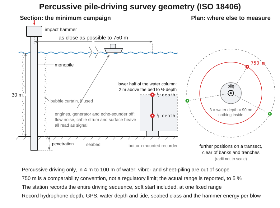
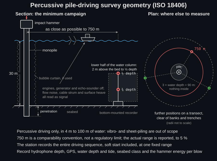
Where the hydrophone goes. The minimum campaign is one measurement position as close as possible to 750 m from the pile, recording the entire driving sequence and reporting the actual range; the standard is explicit that 750 m is chosen for comparability with the large body of existing measurements, not because any regulator’s limit lives there, and that a single-range level has no predictive value for other sites (Clause 6.1.2.1, Notes 1–2). Offshore, the hydrophone sits in the lower half of the water column, between 2 m above the sea floor and half the total depth measured from the surface, because the field is strongly depth-dependent in the upper part of the column (Clause 5.2.1); inshore, in harbours and estuaries, it is fixed at half the water depth (Clause 5.2.2). Two hydrophones are better than one — redundancy, two sensitivities to cover the dynamic range, and spatial averaging — placed at two depths in the lower half, ideally near ½ and ¾ of the total depth with the separation maximised (Clause 5.2.3). Additional positions are no closer than three times the local water depth at the pile, which is also the inshore rule when 750 m is impossible, because closer than that the level depends strongly on the measurement depth (Clauses 6.1.2.2 and 6.1.3.2). The range itself has to be known to 5 % or better (Clause 6.3).

What the instrument has to do. The system frequency range extends from no more than 20 Hz to no less than 20 kHz; the hydrophone is omnidirectional to within 2 dB over that range, and the response flat to within about 2 dB or else calibrated across it (Clauses 4.2.2, 4.2.3). Signal-to-noise is at least 10 dB and the system self-noise at least 10 dB below the lowest level to be measured, which is a real constraint for background work: an ordinary recorder’s self-noise approaches sea-state-zero levels near 63 Hz and 125 Hz (Clauses 4.2.4, 4.2.5). The dynamic range is chosen so the highest expected pressure is recorded without saturation, with over 60 dB preferred (Clause 4.2.6) — the peak level is a regulated metric and clipping destroys it silently while still returning a plausible number.

Calibration. The full chain is calibrated over that frequency range — hydrophone, amplifiers, filters and the ADC’s full-scale setting and calibration factor — traceable to national or international standards, with the hydrophone calibration conforming to IEC 60565; laboratory calibration preferably not more than two years apart, and a pistonphone field check before and after every major deployment (Clauses 4.3.1, 4.3.2). Analyse uncompressed data (Clause 4.4).

What silently ruins a record. Flow noise below about 100 Hz, worst in tidal streams; cable strum when a current pulls a cable taut; surface heave, where a 10 cm change in the water column above a surface-suspended hydrophone is a 1 kPa hydrostatic swing — 180 dB re 1 µPa — that eats the ADC’s range; the measuring vessel’s own engine, generator, inverter and echo-sounder, which are switched off, with the engine condition stated in the results; chains, shackles and cables rubbing; and electrical interference (Clause 5.3). Background noise is measured with the piling stopped, over the same averaging time as the signal, and the signal-to-noise ratio determined from it (Clause 6.1.4).

What the report has to carry. Date and time, hydrophone depth, GPS positions of pile and hydrophones, seabed type with the classification scheme named, water depth and the tidal variation during piling, the measuring vessel’s operating condition and the significant sources of uncertainty (Clause 8.1.2); pile dimensions and material, water depth at the pile, hammer model, the per-blow energy history including the soft start, penetration depth and any mitigation such as a bubble curtain (Clause 8.2); and the deployment configuration with its calibration certificates (Clause 8.3.1). Results are reported per hydrophone and per position: broadband and per-band single-strike SEL, the peak sound pressure level, and the signal-to-noise ratio (Clause 8.4.1). Without that record a single-range SEL says nothing about any other site — which is the point of Notes 1–2 above.

Impact criteria for marine fauna are phrased in exactly the quantities of this section, a cap on the single-strike or cumulative SEL and on the peak level at a stated range, which is why pile_strike_metrics reports them together and cumulative_sel follows the strike-by-strike energy sum of ISO 18406 Formulae 8-9. Turning those numbers into an assessment — weighting the spectrum for a hearing group, accumulating it over the strikes and comparing it against the published onset criteria — is Marine-mammal noise exposure.

What this guide covers

Covered
ISO 18405:2017 for the reference levels re 1 µPa and 1 µPa²·s: sound_pressure_level, sound_exposure_level and peak_sound_pressure_level. ISO 17208-1:2016 and ISO 17208-2:2019 for the ship radiated noise level and the equivalent monopole source level: radiated_noise_level and monopole_source_level, with the Lloyd’s-mirror surface correction (ISO 17208-2 Formula 3) and the 0.7·draught source depth (ISO 17208-2 Formula 1), the three-hydrophone geometry (hydrophone_depths) and the tabulated source-level uncertainty (source_level_uncertainty). ISO 18406:2017 for the pile-driving metrics of section 3: the single-strike SEL (ISO 18406 Formulae 3-4), the mean-square SPL (ISO 18406 Formula 7) and the cumulative SEL (ISO 18406 Formulae 8-9), which single_strike_sel, cumulative_sel, cumulative_sel_identical and pile_strike_metrics compute.
Not covered
ISO 17208-1’s measurement discipline itself is not implemented: the four-run, three-hydrophone power and arithmetic averaging (ISO 17208-1 Formulae 8-9), the CPA and water-depth geometry checks, the ±30° data-window scoring and the ISO 3744-style background-noise correction described in section 2 above are left to the reader; the library only supplies the closed-form radiated_noise_level and monopole_source_level formulae. The same holds for the ISO 18406 survey of section 3: the deployment, instrument, calibration and reporting requirements are described here and enforced nowhere in code, and nothing checks that a strike handed to pile_strike_metrics came from a record that meets them. ISO 18406 itself excludes vibro- and sheet-piling from its scope, and piling in less than 4 m or more than 100 m of water (Clause 1), so continuous pile-driving noise has no closed form here or elsewhere in phonometry.

References

Ainslie, M. A. (2010). Principles of sonar performance modelling. Springer. https://doi.org/10.1007/978-3-540-87662-5The systematic treatment of underwater acoustical quantities in the line that ISO 18405 standardised; supports the reference levels and the source level of sections 1-2.
International Organization for Standardization. (2016). Underwater acoustics — Quantities and procedures for description and measurement of underwater sound from ships — Part 1: Requirements for precision measurements in deep water used for comparison purposes (ISO 17208-1:2016). The radiated noise level, the deep-water three-hydrophone geometry and the tabulated source-level uncertainty of section 2.
International Organization for Standardization. (2017). Underwater acoustics — Measurement of radiated underwater sound from percussive pile driving (ISO 18406:2017). The single-strike (Formulae 3–4), peak and cumulative (Formulae 8–9) sound exposure of section 3, and the mean-square sound pressure level (Formula 7) of section 1.
International Organization for Standardization. (2017). Underwater acoustics — Terminology (ISO 18405:2017). The 1 µPa sound-pressure and 1 µPa²·s sound-exposure references and the definitions of sound pressure level, sound exposure level and peak sound pressure level.
International Organization for Standardization. (2019). Underwater acoustics — Quantities and procedures for description and measurement of underwater sound from ships — Part 2: Determination of source levels from deep water measurements (ISO 17208-2:2019). The equivalent monopole source level via the Lloyd's-mirror surface correction (Formula 3) for a 0.7·draught source depth.
Urick, R. J. (1983). Principles of underwater sound (3rd ed.). McGraw-Hill. Reprinted 1996 by Peninsula Publishing. ISBN 978-0-932146-62-5. Open Library record (https://openlibrary.org/books/OL9317725M). The classic treatment of underwater sound levels and of ship radiated noise behind the reference conventions of sections 1-2.

Created and maintained by José Manuel Requena Plens ORCID All projects