Marine-mammal noise exposure

A marine mammal does not hear every frequency equally, so an underwater noise assessment cannot compare a broadband level against a single number. Regulatory practice instead weights the spectrum with a filter shaped like the hearing group’s sensitivity, sums the weighted energy, accumulates it over the whole activity and compares the result against a published onset criterion — the exposure at which a temporary threshold shift (TTS) in hearing sensitivity begins, and the higher one at which the shift becomes permanent, historically PTS and, since the 2024 guidance, auditory injury (AUD INJ). This page covers the three pieces the library provides for that chain: the hearing curves themselves, the weighting functions and criteria of the current guidance, and the end-to-end assessment of a piling campaign.

Levels are in dB re 1 µPa (sound pressure), dB re 1 µPa²·s (sound exposure) or, for the two in-air carnivore groups, dB re 20 µPa and dB re (20 µPa)²·s. The underwater reference conventions themselves are in Underwater acoustics.

Hearing groups (and why the names collide)

Every current criteria set sorts marine mammals into hearing groups and gives each one a filter. The group codes are not portable between guidance versions, and the collision is a real trap:

Animal group	Southall 2019	NMFS 2024	NMFS 2018	Audiogram
Baleen whales	LF	LF	LF	no ($F_1$ unpublished)
Sperm, beaked and most delphinid whales	HF	HF	MF	yes ("HF")
Porpoises, Cephalorhynchus, Kogia	VHF	VHF	HF	yes ("VHF")
Phocid seals in water	PCW	PW	PW	yes ("PCW")
Otariids in water	OCW	OW	OW	yes ("OCW")
Sirenians	SI	—	—	yes ("SI")
Phocid seals in air	PCA	PA	—	yes ("PCA")
Otariids in air	OCA	OA	—	yes ("OCA")

Read the column you are working in. auditory_weighting and exposure_criteria take the code of the guidance you select; group_audiogram always takes the Southall code, because the audiograms are Southall’s. So group_audiogram(f, "PW") raises even though "PW" is a valid NMFS 2024 weighting group — ask for "PCW" — and auditory_weighting(f, "PCW") raises under the default guidance for the mirror-image reason. hearing_groups(guidance) lists the codes a version defines, and passing a code from the wrong version raises rather than silently returning the wrong filter.

from phonometry import underwater

print(underwater.hearing_groups("nmfs-2024"))
# ('LF', 'HF', 'VHF', 'PW', 'OW', 'PA', 'OA')
print(underwater.hearing_groups("nmfs-2018"))
# ('LF', 'MF', 'HF', 'PW', 'OW')

Group audiograms

group_audiogram evaluates the band-pass fit of Southall et al. (2019), Equation (1), after Finneran (2016):

$$T(f)=T_0+A{\log }_{10}\left(1+\frac{F_1}{f}\right)+(f/F_2{)}^B,$$

with $f$ in kilohertz. normalized=False (the default) uses the Table 2 parameters, fitted to the absolute median behavioural thresholds; normalized=True uses the Table 3 refit on thresholds normalised to each individual’s best value. The article publishes no fitted audiogram for LF cetaceans (no audiometric data exist and $F_1$ is never printed), so that group is deliberately absent rather than reconstructed by guesswork.

import numpy as np
from phonometry import underwater

freqs = np.logspace(2, 5.3, 400)
audiogram = underwater.group_audiogram(freqs, "VHF")
print(audiogram.best_frequency, audiogram.best_threshold)
audiogram.plot()   # threshold vs frequency (needs matplotlib)

print(underwater.AUDIOGRAM_GROUPS)
# ('HF', 'VHF', 'SI', 'PCW', 'OCW', 'PCA', 'OCA')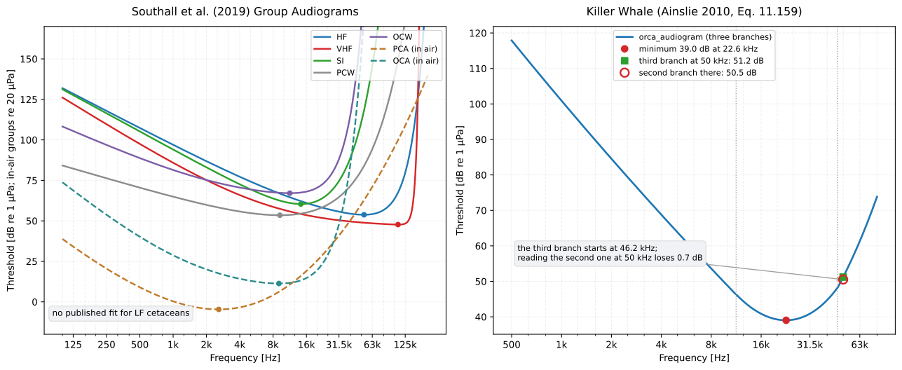

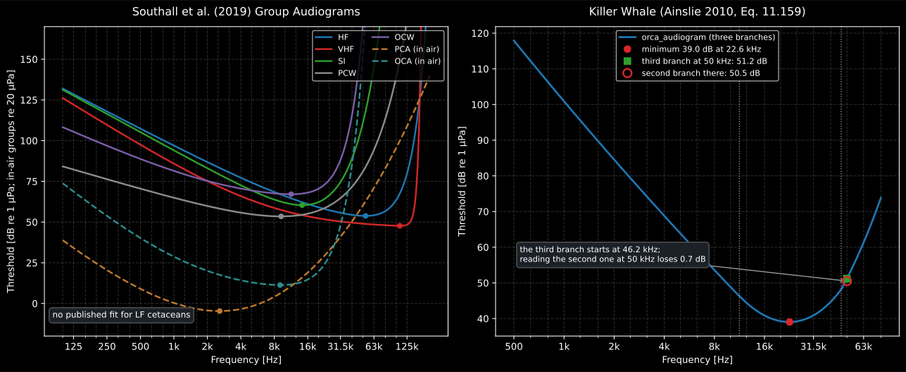
The groups are tens of decibels and more than a decade of best frequency apart: a porpoise hears best near 109 kHz at 48 dB re 1 µPa, a sirenian near 14 kHz at 60 dB. The gap at the left of the panel is the missing LF fit, and it is the reason the weighting section below has a group the audiogram section does not. On the right, the two markers at 50 kHz are 0.7 dB apart and that is the whole point of the branch trap. An AudiogramResult draws itself with audiogram.plot().

Show the code for this figure

import matplotlib.pyplot as plt

fig, (ax_g, ax_o) = plt.subplots(1, 2, figsize=(13.5, 5.6))
f_all = np.logspace(2.0, np.log10(200e3), 700)
for group in underwater.AUDIOGRAM_GROUPS:
    res = underwater.group_audiogram(f_all, group)
    ax_g.semilogx(res.frequencies, res.threshold,
                  "--" if res.in_air else "-", label=group)
    ax_g.plot([res.best_frequency], [res.best_threshold], "o")
ax_g.set_ylim(-20.0, 170.0)
ax_g.set(xlabel="Frequency [Hz]", ylabel="Threshold [dB re 1 uPa]")
ax_g.legend(ncols=2)

f_orca = np.logspace(np.log10(500.0), np.log10(80e3), 600)
orca = underwater.orca_audiogram(f_orca)
ax_o.semilogx(orca.frequencies, orca.threshold, label="orca_audiogram")
ax_o.plot([orca.best_frequency], [orca.best_threshold], "o")
ax_o.plot([50e3], [underwater.orca_audiogram(50e3).threshold[0]], "s")
# What the second branch would have returned at 50 kHz, from the printed fit.
ax_o.plot([50e3], [242.9 * 50.0 ** -0.7578 + 0.5643 * 50.0**1.076],
          "o", markerfacecolor="none")
ax_o.set(xlabel="Frequency [Hz]", ylabel="Threshold [dB re 1 uPa]")
ax_o.legend()
plt.show()

For a species rather than a group, orca_audiogram implements the killer-whale curve of Wensveen & Van Roij (2007) as printed in Ainslie (2010), Equation (11.159), a three-branch power law over 0.5 to 80 kHz. Its minimum is 39.0 dB re 1 µPa at 22.6 kHz, and 51.2 dB re 1 µPa at 50 kHz. That second value needs the third branch: evaluating the second one there returns 50.5 dB instead, which is why both published points are pinned by the tests.

from phonometry import underwater

print(underwater.orca_audiogram(50e3).threshold[0])   # 51.20 dB re 1 uPa

That value is the hearing threshold $HT$ in Ainslie’s orca-versus-salmon example. An echolocating orca is an active sonar: it pays the propagation loss twice, so with a source level $SL=198.2$ dB re 1 µPa²m², a salmon target strength $TS=-29.0$ dB re m² and its own hearing threshold in place of a detection threshold, the hearing-limited figure of merit is $(SL+TS-HT)/2=59.0$ dB re m² — the maximum one-way loss it can afford. The sonar equation those terms come from, and detection_range, turn that figure into a range.

Auditory weighting and exposure functions

An audiogram and a weighting function look alike and answer different questions, and substituting one for the other is a common error in assessments. An audiogram is a detection threshold, measured behaviourally or by evoked potential; it answers questions about audibility, masking and detection range — the orca-versus-salmon figure of merit above is exactly that kind of question. A weighting function is fitted to susceptibility data, the frequency dependence of temporary threshold shift, and it is the only one of the two that may be applied to an exposure before comparing it against a TTS or injury criterion. The two curves are not the same shape, because the frequency at which an animal hears best is not always the frequency at which it is most easily damaged, and an inverted audiogram is not a legitimate weighting function. That distinction also resolves the asymmetry between these two sections: LF cetaceans have a weighting function derived from modelled susceptibility, and no fitted audiogram, because no audiometric data exist for baleen whales.

All three current criteria sets use the same generic band-pass filter (NMFS 2018 Equation 1, Southall et al. Equation 2):

$$W(f)=C+10{\log }_{10}\frac{(f/f_1{)}^{2a}}{{\left[1+(f/f_1{)}^2\right]}^a{\left[1+(f/f_2{)}^2\right]}^b},$$

with $f$ in kilohertz. $C$ is fixed by putting the peak of $W$ at 0 dB, so the companion exposure function $E(f)=K+C-W(f)$ has its minimum at the weighted TTS-onset threshold $T_w=K+C$. Below $f_1$ the filter falls at $20a$ dB/decade and above $f_2$ at $20b$ dB/decade.

Only the parameter table changes between versions, so the version is an explicit argument and is carried on the result:

• "nmfs-2024" (the default): NOAA Fisheries Updated Technical Guidance v3.0, October 2024. It supersedes the 2018 revision, sets $b=5$ for every group, adopts the Southall group names and replaces “PTS onset” with “auditory injury (AUD INJ) onset”.
• "nmfs-2018": the 2018 revision v2.0, still cited by assessments already in flight.
• "southall-2019": the peer-reviewed criteria, numerically identical to NMFS 2018 on the five shared groups and adds sirenians and both in-air carnivore groups.

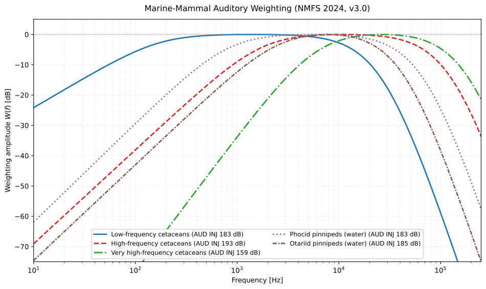
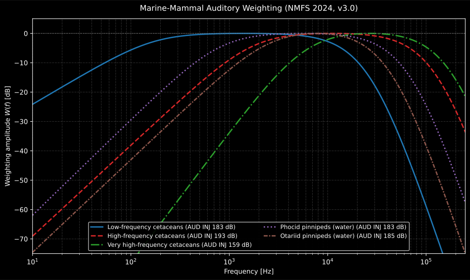
Five band-passes of the same algebraic form, and choosing the wrong one costs more than the criterion itself does. At 1 kHz — where a pile drive or a ship puts most of its energy — the LF filter is at −0.03 dB and the VHF filter at −33.84 dB, so the same measured spectrum yields two weighted exposures 34 dB apart before any threshold is applied. The −6 dB passbands barely overlap (96 Hz-15 kHz for LF against 5.9-113 kHz for VHF), and the AUD INJ thresholds in the legend run from 159 to 193 dB, so group and criterion have to be quoted together or the number means nothing.

Show the code for this figure

import matplotlib.pyplot as plt
import numpy as np
from phonometry import underwater

freqs = np.logspace(1, 5.4, 700)
fig, ax = plt.subplots()
for group in ("LF", "HF", "VHF", "PW", "OW"):
    res = underwater.auditory_weighting(freqs, group, guidance="nmfs-2024")
    crit = underwater.exposure_criteria(group, guidance="nmfs-2024", impulsive=True)
    ax.semilogx(res.frequencies, res.weighting,
                label=f"{group} (AUD INJ {crit.injury_sel:.0f} dB)")
ax.set(xlabel="Frequency [Hz]", ylabel="Weighting amplitude W(f) [dB]",
       ylim=(-75, 5))
ax.legend()
ax.grid(True, which="both", alpha=0.3)
plt.show()

from phonometry import underwater

res = underwater.auditory_weighting(1000.0, "LF", guidance="nmfs-2018")
print(res.weighting[0])           # -0.06 dB, the published Appendix D value
print(res.weighted_tts_onset)     # Tw = K + C

params = underwater.weighting_parameters("OW", guidance="nmfs-2024")
print(params.a, params.b, params.f1_khz, params.f2_khz, params.c_db)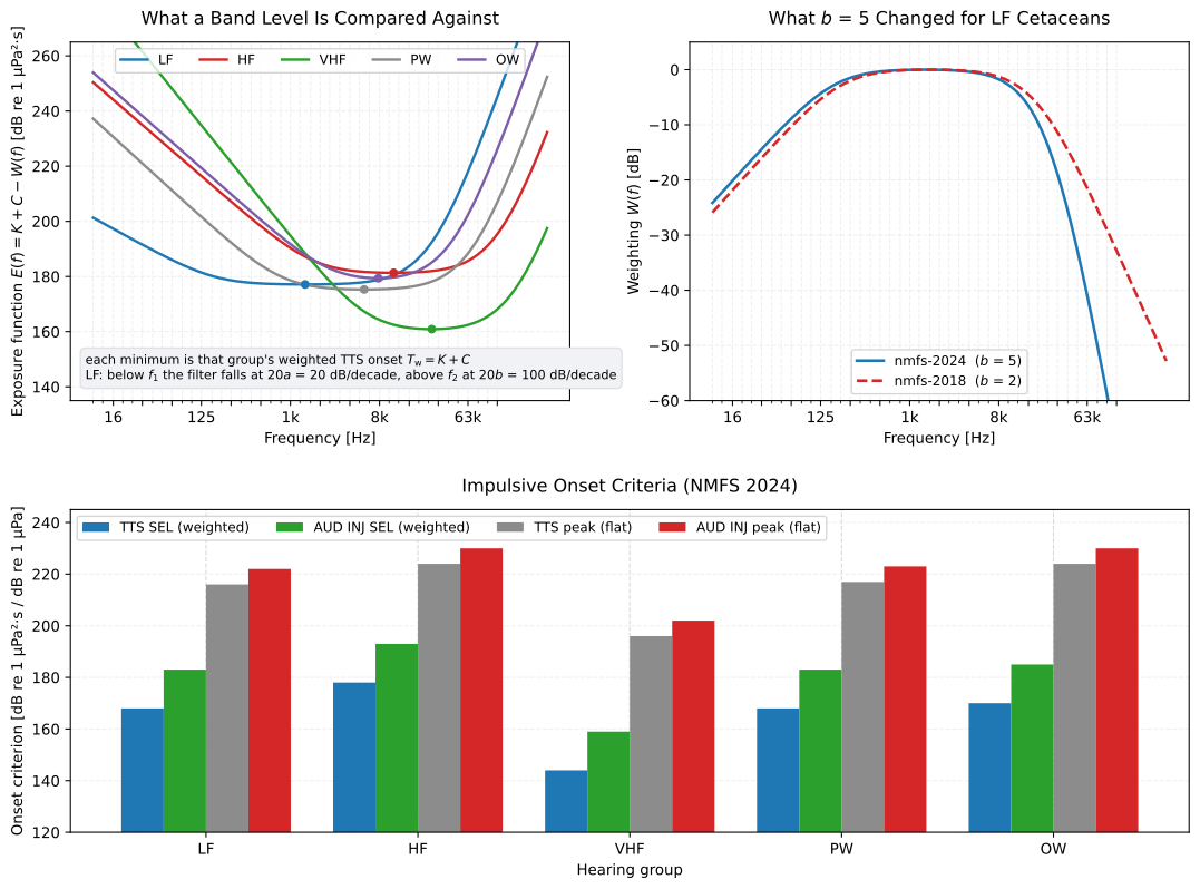

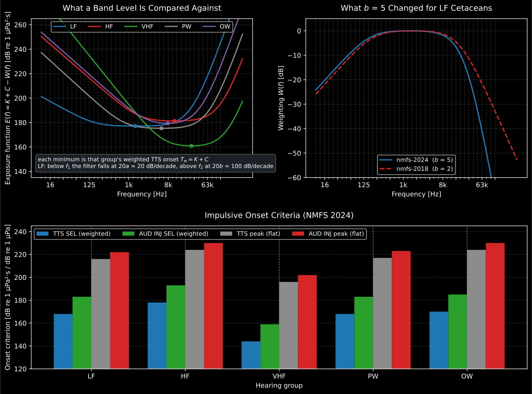
Note

NMFS 2024 prints $C=1.37$ dB for the otariid in-water group and states in the same table’s footnote that the value should be 1.36 dB. The library implements 1.36 (recomputing $C$ from the peak of $W$ gives 1.3643) and keeps the printed digit as c_db_as_printed. Southall’s Table 7 carries four peak-SPL misprints corrected by the journal’s own errata, and the corrected values are the ones implemented. Both are recorded in Errata found in published sources.

The exposure function is what a measured band level is actually compared against: a threshold spectrum whose minimum is the group’s weighted TTS onset $T_w=K+C$. The 2024 revision set $b=5$ for every group, which steepens the high-frequency skirt from 40 to 100 dB/decade and therefore discounts energy above $f_2$ far more heavily than the 2018 tables did. The bars show why the group matters more than anything else in the chain: the porpoise group’s weighted TTS onset is 24 dB below the low-frequency cetacean’s, and its peak criterion 20 dB below.

Show the code for this figure

import matplotlib.pyplot as plt

f_w = np.logspace(1.0, np.log10(400e3), 800)
groups = ("LF", "HF", "VHF", "PW", "OW")
fig = plt.figure(figsize=(13.5, 9.6))
gs = fig.add_gridspec(2, 2, height_ratios=[1.0, 0.9], hspace=0.32, wspace=0.24)
ax_e, ax_w, ax_c = (fig.add_subplot(gs[0, 0]), fig.add_subplot(gs[0, 1]),
                    fig.add_subplot(gs[1, :]))

for group in groups:
    res = underwater.auditory_weighting(f_w, group, guidance="nmfs-2024")
    exposure = np.asarray(res.exposure_function)
    ax_e.semilogx(res.frequencies, exposure, label=group)
    ax_e.plot([res.frequencies[int(np.argmin(exposure))]], [exposure.min()], "o")
ax_e.set_ylim(135.0, 265.0)
ax_e.set(xlabel="Frequency [Hz]", ylabel="E(f) = K + C - W(f) [dB re 1 uPa^2 s]")
ax_e.legend(ncols=5)

for guidance in ("nmfs-2024", "nmfs-2018"):
    res = underwater.auditory_weighting(f_w, "LF", guidance=guidance)
    ax_w.semilogx(res.frequencies, res.weighting,
                  label=f"{guidance} (b = {res.parameters.b:g})")
ax_w.set_ylim(-60.0, 5.0)
ax_w.set(xlabel="Frequency [Hz]", ylabel="Weighting W(f) [dB]")
ax_w.legend()

idx = np.arange(len(groups), dtype=float)
for offset, attr in ((-1.5, "tts_sel"), (-0.5, "injury_sel"),
                     (0.5, "tts_peak_spl"), (1.5, "injury_peak_spl")):
    ax_c.bar(idx + offset * 0.2,
             [getattr(underwater.exposure_criteria(g, guidance="nmfs-2024",
                                                   impulsive=True), attr)
              for g in groups], 0.2, label=attr)
ax_c.set_xticks(idx, groups)
ax_c.set_ylim(120.0, 245.0)
ax_c.set(xlabel="Hearing group", ylabel="Onset criterion [dB]")
ax_c.legend(ncols=4)
plt.show()

Onset criteria

exposure_criteria returns the published TTS and injury onset criteria of a group. Impulsive noise carries a dual metric: a weighted sound exposure level and an unweighted (“flat”) peak sound pressure level, and the criterion that produces the larger isopleth governs — the isopleth being the contour on which the criterion is exactly met, so the metric that pushes it furthest from the source is the one that sets the mitigation zone.

from phonometry import underwater

crit = underwater.exposure_criteria("VHF", guidance="nmfs-2024", impulsive=True)
print(crit.injury_label)        # 'AUD INJ'
print(crit.tts_sel, crit.injury_sel)          # 144, 159 dB re 1 uPa2 s (weighted)
print(crit.tts_peak_spl, crit.injury_peak_spl)  # 196, 202 dB re 1 uPa (flat)
print(crit.source)

The impulsive criteria of the five in-water groups, under the default guidance, are the numbers most readers come here for:

Group	TTS SEL (weighted)	AUD INJ SEL (weighted)	TTS peak (flat)	AUD INJ peak (flat)
LF	168	183	216	222
HF	178	193	224	230
VHF	144	159	196	202
PW	168	183	217	223
OW	170	185	224	230

The SEL columns are dB re 1 µPa²·s and the peak columns dB re 1 µPa; the in-air groups PA and OA come from the same call and use 20 µPa references. The non-impulsive criteria drop the peak columns entirely and sit on their own TTS values plus 20 dB (LF 177 → 197, VHF 161 → 181), so they are not the impulsive numbers with a column removed.

The tables are internally consistent in ways the library pins as tests: the non-impulsive injury level is always TTS + 20 dB, the published weighted TTS onset is always the rounded $K+C$, and in Southall’s impulsive table the SEL criteria run TTS + 15 dB and the peak criteria TTS + 6 dB — which the table above satisfies row by row.

A worked pile-driving assessment

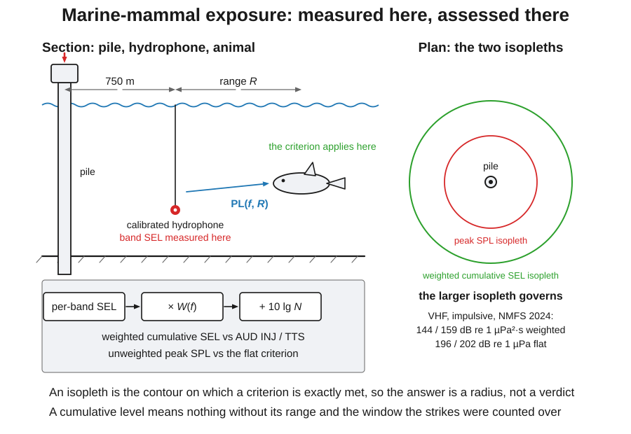
Percussive pile driving is the canonical impulsive case. The chain runs from the recorded strike to the verdict:

1. strike_sel_spectrum splits the single-strike sound exposure of the record into fractional-octave bands (the band energies sum back to the broadband single_strike_sel of Underwater acoustics, by Parseval);
2. weighted_exposure applies $W(f)$ band by band, sums the weighted energy, accumulates it over the number of strikes (the ISO 18406 $+10{\log }_{10}N$) and compares the result with the criteria, unweighted peak SPL included.

What the recording has to cover

The weighted sum runs over the bands it is handed, so the record must span the hearing group’s passband. The NMFS 2024 upper transition frequencies $f_2$ are 26.6 kHz (LF), 129 kHz (HF), 186 kHz (VHF), 68.3 kHz (PW) and 43.8 kHz (OW), and the generalised hearing ranges reach further still (LF to 36 kHz, VHF to 165 kHz). As a rule the sample rate has to be about 2.5 times the highest band edge that matters, so the 48 kHz record below — bands resolved to roughly 20 kHz — supports LF, is marginal for OW, and truncates HF, VHF and PW badly. A porpoise assessment needs a few hundred kilohertz.

weighted_exposure cannot detect a truncated spectrum: it weights what it is given, so a short record simply reports a lower cumulative SEL and no warning. The unweighted peak half of the dual metric has to come from the same record with no clipping and headroom to spare, which is why ISO 18406 makes dynamic range a survey requirement: a saturated capture reads as a compliant peak.

import numpy as np
from phonometry import underwater

# One recorded strike (here a synthetic 200 Hz decaying burst). 48 kHz is
# enough for the LF group used below and for nothing above it.
fs = 48_000
t = np.arange(int(0.2 * fs)) / fs
strike = 50.0 * np.exp(-t / 0.06) * np.sin(2 * np.pi * 200.0 * t)

spectrum = underwater.strike_sel_spectrum(strike, fs, fraction=3)
peak = underwater.peak_sound_pressure_level(strike)

res = underwater.weighted_exposure(
    spectrum.frequencies, spectrum.band_sel, "LF",
    guidance="nmfs-2024", impulsive=True, n_events=3000, peak_spl=peak,
)
print(res.unweighted_sel, res.weighted_sel, res.cumulative_sel)
print(res.sel_margin, res.peak_margin)       # positive means the criterion is exceeded
print(res.exceeds_injury, res.exceeds_tts)
res.plot()   # weighted spectrum against the criteria (needs matplotlib)

Read those six numbers in order, because each one is a step. The record’s unweighted single-strike exposure is 135.7 dB re 1 µPa²·s; LF weighting takes it to 133.5 dB, costing barely 2 dB, because a 200 Hz hammer sits inside the low-frequency cetacean passband. Accumulating 3 000 strikes adds $10{\log }_{10}3000=34.8$ dB and gives 168.3 dB — that term, not the weighting, is what usually decides the outcome. The margins are then read against the criteria: sel_margin = −14.7 dB against the 183 dB auditory injury criterion, so exceeds_injury is False, but the cumulative level clears the 168 dB TTS onset by three tenths of a decibel, so exceeds_tts is True. The flat peak of this record is 153.8 dB re 1 µPa, peak_margin = −68.2 dB, nowhere near the 222 dB peak criterion.

Those are the magnitudes of a synthetic strike, and they are quiet. Measured percussive piling at the standard 750 m position runs to peak levels of order 200 dB re 1 µPa and single-strike exposures of order 175-180 dB re 1 µPa²·s, so a real pile approaches the low-frequency injury criterion of 183 dB while staying far below it once VHF weighting is applied. A result far outside those ranges is a units or calibration error rather than an unusual pile.

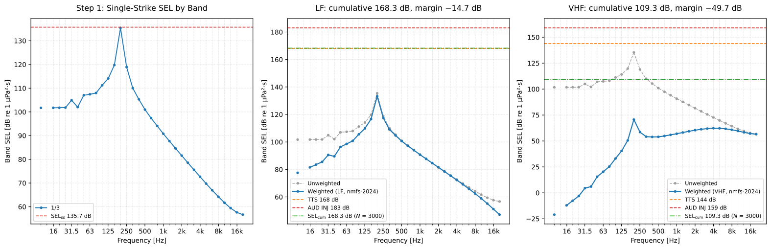
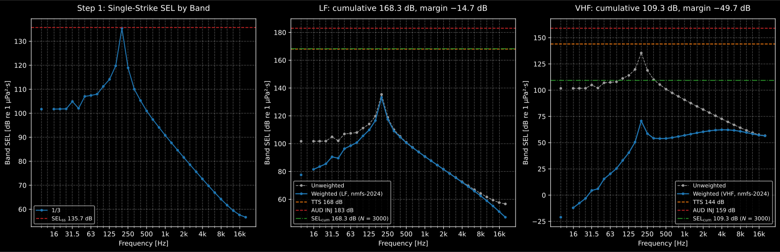
The same campaign, judged twice. For a baleen whale the weighting costs 2 dB and the cumulative level lands between the two criteria; for a porpoise the weighting costs 59 dB and the same piling sits 50 dB below its injury criterion. That is the whole point of weighting, and the reason a single unweighted cumulative SEL is not an assessment. res.plot() draws either panel.

Show the code for this figure

import matplotlib.pyplot as plt

fig, axes = plt.subplots(1, 3, figsize=(16.5, 5.4))
spectrum.plot(ax=axes[0])
for ax, group in zip(axes[1:], ("LF", "VHF"), strict=True):
    verdict = underwater.weighted_exposure(
        spectrum.frequencies, spectrum.band_sel, group,
        guidance="nmfs-2024", impulsive=True, n_events=3000, peak_spl=peak)
    verdict.plot(ax=ax)
    ax.set_title(f"{group}: cumulative {verdict.cumulative_sel:.1f} dB, "
                 f"margin {verdict.sel_margin:+.1f} dB")
plt.show()

The operational question a campaign asks is not “does 3 000 strikes exceed the criterion” but “how many strikes may be driven, and which group binds first”. That is one loop over weighted_exposure with a rising n_events.

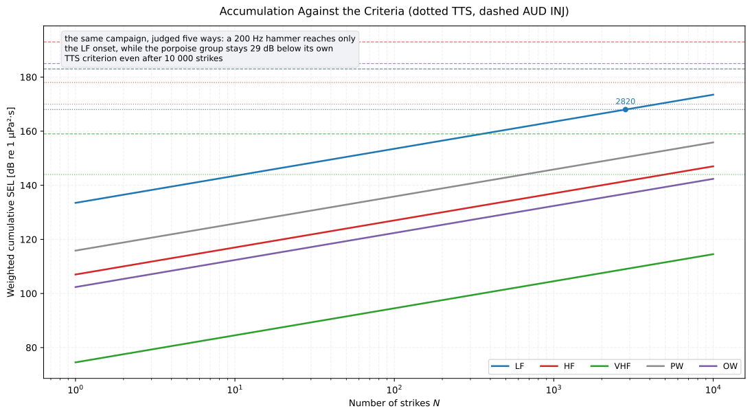
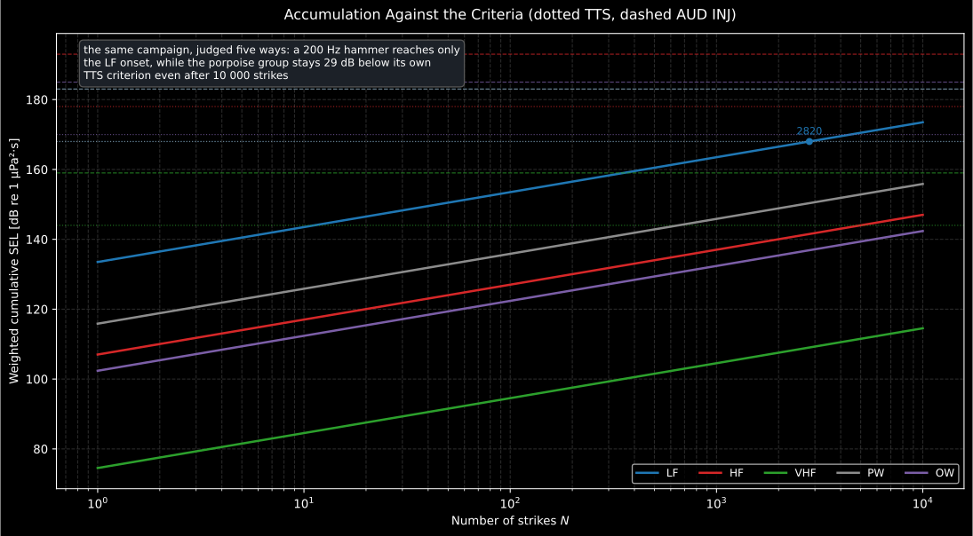
Every curve is a straight line on a log-N axis, because accumulation adds $10{\log }_{10}N$ and nothing else: the group decides the intercept and the strike count decides the rest. For this 200 Hz hammer only the low-frequency group reaches a criterion at all, at 2 820 strikes, and no group reaches its injury criterion within 10 000. The curve is a stationary-receiver worst case: the library does not move the animal.

Show the code for this figure

import matplotlib.pyplot as plt

counts = np.unique(np.round(np.logspace(0.0, 4.0, 90)).astype(int))
fig, ax = plt.subplots(figsize=(11.5, 6.4))
for group in ("LF", "HF", "VHF", "PW", "OW"):
    curve = [underwater.weighted_exposure(
        spectrum.frequencies, spectrum.band_sel, group, guidance="nmfs-2024",
        impulsive=True, n_events=int(n)).cumulative_sel for n in counts]
    line, = ax.semilogx(counts, curve, label=group)
    crit = underwater.exposure_criteria(group, guidance="nmfs-2024",
                                        impulsive=True)
    ax.axhline(crit.tts_sel, color=line.get_color(), linestyle=":")
    ax.axhline(crit.injury_sel, color=line.get_color(), linestyle="--")
ax.set(xlabel="Number of strikes N",
       ylabel="Weighted cumulative SEL [dB re 1 uPa^2 s]")
ax.legend(ncols=5)
plt.show()

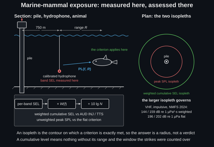
From a criterion to an isopleth

A margin is not the regulatory output; a distance is. An isopleth is the locus on which a criterion is exactly met, so the answer an assessment owes is a radius: the range beyond which the accumulated weighted SEL no longer exceeds its criterion, and separately the range beyond which the flat peak no longer exceeds its own, with the larger of the two governing.

The bridge from this page to that radius runs through the propagation guide. Take the band SEL at the range it was measured at — 750 m, per ISO 18406 — propagate it to a trial range with propagation_loss at each band centre, re-run weighted_exposure on the propagated spectrum for the strike count of the campaign, and read off the range where sel_margin crosses zero. Then repeat for the flat peak, where only the single-trip loss applies.

def band_loss(r):
    """Per-band propagation loss at range r, in 30 m of water."""
    return np.array([float(underwater.propagation_loss(
        r, float(f), law="practical", transition_range=30.0).pl[0])
        for f in spectrum.frequencies])

reference = band_loss(750.0)          # the range the strike was measured at
for r in (750.0, 800.0, 1000.0, 3000.0):
    out = underwater.weighted_exposure(
        spectrum.frequencies, spectrum.band_sel - (band_loss(r) - reference),
        "LF", guidance="nmfs-2024", impulsive=True, n_events=3000,
        peak_spl=peak)
    print(int(r), round(out.cumulative_sel, 1), round(out.tts_margin, 2))
# 750 168.3 0.27   <- exceeded
# 800 168.0 -0.01  <- the TTS isopleth is here
# 1000 167.0 -0.98
# 3000 162.2 -5.76

For this campaign the low-frequency TTS isopleth sits at about 800 m, and there is no injury isopleth at all: the cumulative level is 14.7 dB below the 183 dB criterion even at the measurement range. The peak isopleth does not exist either, for the same reason — which is exactly the case where the larger isopleth rule has nothing to choose between, and the assessment reduces to one radius.

Two consequences follow, and both belong in the report. The governing metric can change with range, because the accumulated SEL carries the $+10{\log }_{10}N$ term and the peak does not, so the two isopleths shrink at different rates. And a cumulative number means nothing without two facts attached: the range at which the strike was measured or modelled, and the accumulation window — 3 000 strikes means one pile driven inside that window, conventionally 24 hours in the regulatory guidance, not a whole campaign.

What this guide covers

• Covered

  group_audiogram and audiogram_parameters implement the Southall et al. (2019) group audiogram (Equation 1) with the Table 2 absolute and Table 3 normalised fits; orca_audiogram implements the three-branch killer-whale audiogram of Ainslie (2010) Equation (11.159). auditory_weighting implements the band-pass weighting and exposure functions for the three selectable guidance versions (NMFS 2024 v3.0, the default; NMFS 2018 v2.0; Southall et al. 2019), with the parameter tables addressable through weighting_parameters. exposure_criteria returns the published TTS and injury (PTS / AUD INJ) onset criteria, impulsive and non-impulsive, including the unweighted peak-SPL half of the dual metric. weighted_exposure runs the assessment: weighting a band spectrum, accumulating it over events and reporting the margin against every applicable criterion. strike_sel_spectrum supplies that band spectrum from a recorded pile strike.

• Not covered

  There is no audiogram for LF cetaceans, because Southall et al. never print its $F_1$ parameter. Behavioural-disturbance criteria (the step-function and dose-response thresholds used for harassment take estimates) are out of scope: only the auditory-effect criteria are implemented. The library does not choose a hearing group or an accumulation period for you, and it does not model the animal’s movement relative to the source, so the cumulative SEL it reports is the stationary-receiver worst case. It also does not check that the supplied spectrum spans the group’s passband: a record that stops short of $f_2$ is weighted as given and under-reports the exposure. Propagation from source to receiver belongs to Underwater sound propagation.

See also

• Underwater acoustics: radiated noise and pile driving: the ISO 18405 reference levels and the ISO 18406 pile-driving exposure that feed this page.
• Underwater sound propagation: the propagation loss and figure-of-merit machinery that turns a criterion into a range.
• API reference: underwater.bioacoustics.weighting and underwater.bioacoustics.audiograms.

References

• Ainslie, M. A. (2010). Principles of Sonar Performance Modelling. Springer/Praxis. https://doi.org/10.1007/978-3-540-87662-5The orca audiogram (Equation 11.159, after Wensveen & Van Roij 2007) and the orca-versus-salmon worked example.
• Finneran, J. J. (2016). Auditory weighting functions and TTS/PTS exposure functions for marine mammals exposed to underwater noise (Technical Report 3026). SSC Pacific. The band-pass filter form and the audiogram equation that both criteria sets adopt.
• International Organization for Standardization. (2017). Underwater acoustics — Terminology (ISO 18405:2017). The symbols and references the guidance documents adopt for their criteria (Lp,0-pk and LE,p re 1 µPa and 1 µPa²·s).
• National Marine Fisheries Service. (2018). 2018 Revision to: Technical Guidance for Assessing the Effects of Anthropogenic Sound on Marine Mammal Hearing (Version 2.0) (NOAA Technical Memorandum NMFS-OPR-59). National Oceanic and Atmospheric Administration. The Table 3 weighting parameters, the Table ES3 PTS onset thresholds and the Appendix D worked example (W at 1 kHz for the five hearing groups) used as the numeric oracle of the weighting section.
• National Marine Fisheries Service. (2024). 2024 Update to: Technical Guidance for Assessing the Effects of Anthropogenic Sound on Marine Mammal Hearing (Version 3.0) (NOAA Technical Memorandum NMFS-OPR-71). National Oceanic and Atmospheric Administration. The current guidance and the library default: Table 5 weighting parameters, Table ES3 AUD INJ criteria and the Navy Phase 4 Table A.E-2 impulsive TTS thresholds.
• Southall, B. L., Finneran, J. J., Reichmuth, C., Nachtigall, P. E., Ketten, D. R., Bowles, A. E., Ellison, W. T., Nowacek, D. P., & Tyack, P. L. (2019). Marine mammal noise exposure criteria: Updated scientific recommendations for residual hearing effects. Aquatic Mammals, 45(2), 125-232. https://doi.org/10.1578/AM.45.2.2019.125The group audiograms (Equation 1 with Tables 2 to 4) and the weighting and threshold tables (Tables 5 to 7); its errata in 45(5), 569-572 corrects four peak-SPL values of Table 7.