Atmospheric refraction: rays and the GFPE

The ISO 9613-2 method and the spherical-wave ground effect both assume a homogeneous atmosphere. In reality the sound speed changes with height, because temperature and wind change with height, and this refracts sound: rays curve, and over a few hundred metres the received level can swing by tens of decibels. This page covers phonometry.environment.propagation.refraction, the refracting-atmosphere counterpart of the ocean solvers in phonometry.underwater.propagation.numerical: a ray model and a parabolic-equation (PE) solver.

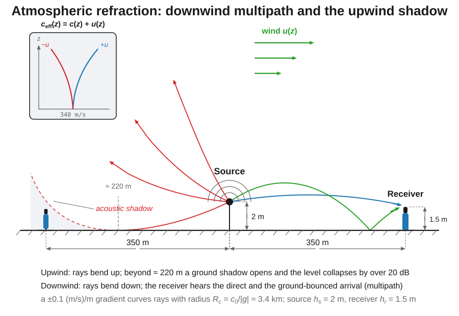
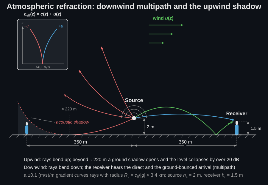
Whether refraction matters is mostly a question of range. A representative surface-layer gradient of ±0.1 s⁻¹ curves rays with a radius $R_c=c_0/|g|\approx 3.4$ km, so over the first hundred metres the paths are sensibly straight and the homogeneous models above are accurate. Beyond a few hundred metres the geometry takes over: downwind, or under a nocturnal temperature inversion, the downward-curved rays close over the ground and hold the level near (or even above) the homogeneous prediction, while upwind the same wind profile opens an acoustic shadow into which the level collapses by 20 dB or more (Attenborough & Van Renterghem 2021, Ch. 11). That is the familiar upwind/downwind asymmetry of any steady outdoor source: the same machine at the same distance, tens of decibels apart depending on which side you stand. It is also why ISO 9613-2 fixes its “favourable” downwind atmosphere by decree, and what its scalar $C_{met}$ compresses; the models on this page compute the physics that decides both.

The sketch below puts both sides in one scene: one source, a receiver 350 m away on each side, and the wind profile deciding which of them hears anything.

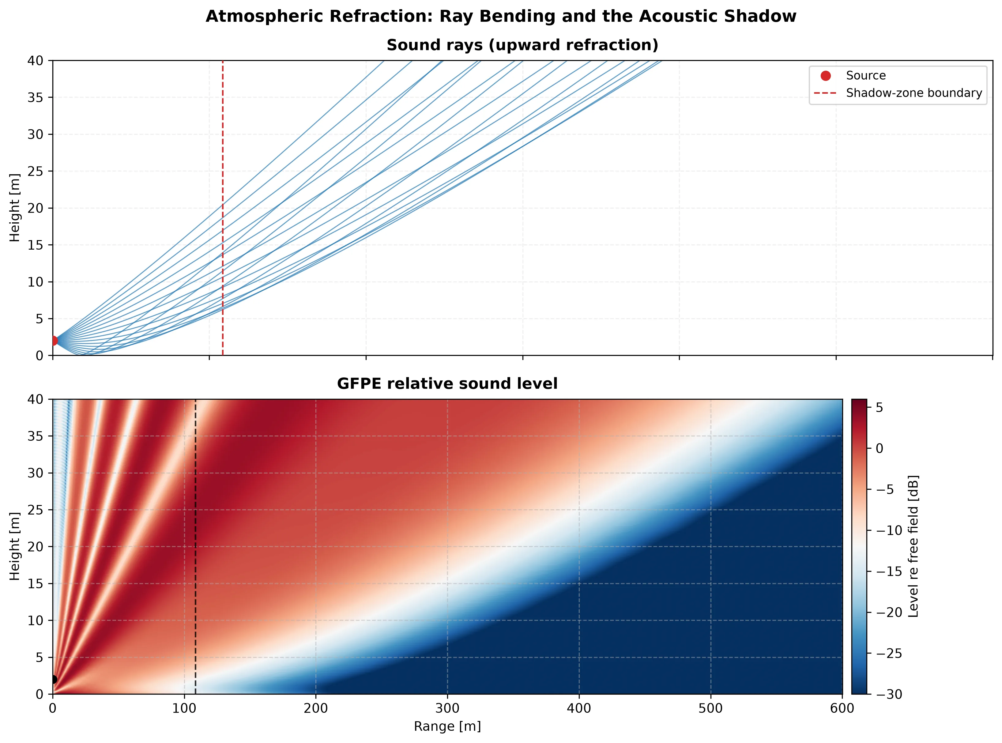
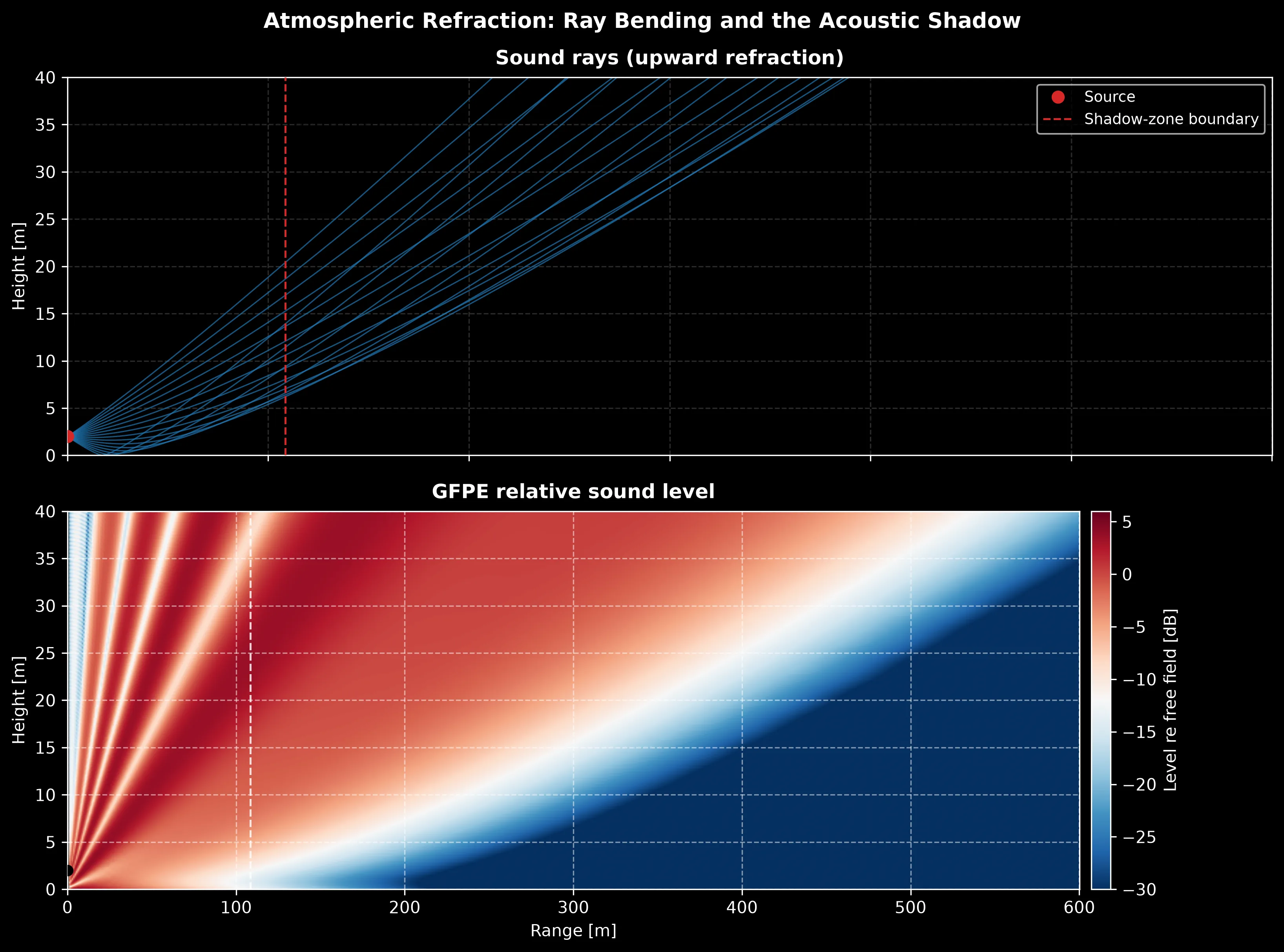
The two halves of the same atmosphere. The ray fan says where the shadow starts — every ray has left the ground by about 110 m — and the GFPE field says how deep it is once you are inside it. Neither picture exists in an octave-band engineering method: this is what $C_{met}$ replaces with one number.

Show the code for this figure

import warnings

import matplotlib.pyplot as plt
import numpy as np

from phonometry import (
    atmospheric_parabolic_equation,
    atmospheric_ray_paths,
    log_linear_sound_speed_profile,
    shadow_zone_distance,
)

c0 = 340.0
profile = log_linear_sound_speed_profile(-1.0, ground_speed=c0, max_height=60.0)
zs = 2.0
fig, axes = plt.subplots(2, 1, figsize=(11, 8.2), sharex=True)

rays = atmospheric_ray_paths(profile, source_height=zs,
                             launch_angles_deg=np.linspace(-8.0, 8.0, 17),
                             max_range=600.0, n_steps=3000)
for i in range(rays.heights.shape[0]):
    axes[0].plot(rays.ranges[i], rays.heights[i], color="#1f77b4", lw=0.8, alpha=0.7)
axes[0].plot([0.0], [zs], "o", color="#d62728", label="Source")
grad = (profile.speed_at(10.0) - c0) / 10.0
x_sh = shadow_zone_distance(float(grad), zs, zs, ground_speed=c0)
axes[0].axvline(x_sh, color="#d62728", ls="--", label="Shadow-zone boundary")
axes[0].set(ylabel="Height [m]", ylim=(0, 40), title="Sound rays (upward refraction)")
axes[0].legend()

with warnings.catch_warnings():
    # The PorousAbsorberWarning: a 200 kPa.s/m2 ground runs the one-parameter
    # impedance model below its published fit range, as every outdoor ground
    # does (see "Choosing the ground impedance" in the ground-effect guide).
    warnings.simplefilter("ignore")
    pe = atmospheric_parabolic_equation(400.0, profile, source_height=zs,
                                        flow_resistivity=200e3,
                                        max_range=600.0, max_height=40.0)
img = axes[1].imshow(pe.relative_level, cmap="RdBu_r", vmin=-30, vmax=6,
                     aspect="auto", origin="lower", interpolation="bilinear",
                     extent=(pe.ranges[0], pe.ranges[-1], pe.heights[0], pe.heights[-1]))
axes[1].axvline(x_sh, color="k", ls="--")
axes[1].set(ylabel="Height [m]", xlabel="Range [m]", ylim=(0, 40),
            title="GFPE relative sound level")
fig.colorbar(img, ax=axes[1], label="Level re free field [dB]")
plt.tight_layout()
plt.show()

1. Effective sound-speed profile

A moving (windy) atmosphere is well approximated by a non-moving one with the effective sound speed $c_{\text{eff}}(z)=c(z)+u(z)$, the adiabatic sound speed plus the component of the wind in the propagation direction (Salomons Eq. 4.4). Two profile shapes cover most surface-layer cases:

• a linear profile $c_{\text{eff}}(z)=c_0+gz$ (linear_sound_speed_profile), the simplest refracting atmosphere and the one with exact ray geometry;
• the realistic logarithmic surface-layer profile $c_{\text{eff}}(z)=c_0+b\ln (1+z/z_0)$ (log_linear_sound_speed_profile, Salomons Eq. 4.5), with $b\approx +1\text{m/s}$ for a typical downward-refracting atmosphere, $b\approx -1\text{m/s}$ for an upward-refracting one, and $z_0$ the roughness length (about 0.1 m for grassland).

A positive gradient (sound speed increasing upward) bends rays down toward the receiver (favourable propagation); a negative gradient bends them up and opens an acoustic shadow near the ground.

Setting b and z0 from a site

$b$ is not a taste setting. The effective profile is $c_{\text{eff}}(z)=\sqrt{\gamma R_{\text{gas}}T(z)}+u_{SR}(z)$ (Attenborough & Van Renterghem 2021, Eq. 1.18), so the coefficient of the logarithmic term follows from a wind speed measured at a stated height once $z_0$ is fixed: matching the profile at that height gives $b=u_{SR}(z_1)/\ln (1+z_1/z_0)$. A 10 m mast reading of 4 m/s blowing straight down the propagation path over grassland ($z_0=0.1$ m) therefore gives $b=4/\ln (101)=0.87$ m/s — close to the “+1 m/s typical” above, and log_linear_sound_speed_profile(0.867) duly returns 344.0 m/s at 10 m.

Only the component along the propagation direction enters $c_{\text{eff}}$: $u_{SR}(z)=u(z)\cos (\pi -\alpha )$ with $\alpha$ the angle between the meteorological wind direction (the direction the wind blows from) and the direction the sound travels (Eq. 1.19). The same 4 m/s at 60° to the path is worth 2 m/s along it, so $b=0.43$ m/s downwind and $-0.43$ m/s upwind — one wind, two atmospheres, which is the whole upwind/downwind asymmetry in one line of arithmetic. It is also the physics behind the ISO 9613-2 favourable-condition window (wind within ±45° of the source-receiver line at 1 to 5 m/s measured 3 to 11 m above ground), quoted in full on Outdoor Sound Propagation.

Temperature has no direction, which is why a clear calm night refracts downward in every direction. Near 10 °C the sound speed changes by about 0.6 m/s per kelvin, so a 2 K inversion between the ground and 10 m contributes $b_T\approx 1.2/\ln (101)=0.26$ m/s with no wind at all. Wind and temperature add: a light downwind breeze on an inversion night is the classic complaint condition.

$z_0$ is a property of the cover, not of the weather. Attenborough & Van Renterghem quote a range from 0.0002 m for still water to about 0.1 m for grass (§1.4), use 0.02 m for the worked profiles of their Figure 1.20, and estimate 0.1 m for the meteorological tower whose year of data they fit with this profile shape; rougher covers — crops with scattered obstacles, hedgerows, scrub, suburban terrain — run from a few tenths of a metre to about 1 m and are best taken from the Davenport roughness classification. The default roughness_length=0.1 of log_linear_sound_speed_profile is the grassland value, so it is the one argument to change first when the site is not a field.

from phonometry import log_linear_sound_speed_profile

profile = log_linear_sound_speed_profile(-1.0, ground_speed=340.0)  # upward
profile.speed_at(10.0)   # effective sound speed 10 m above the ground
profile.plot()           # c_eff(z) with height on the vertical axis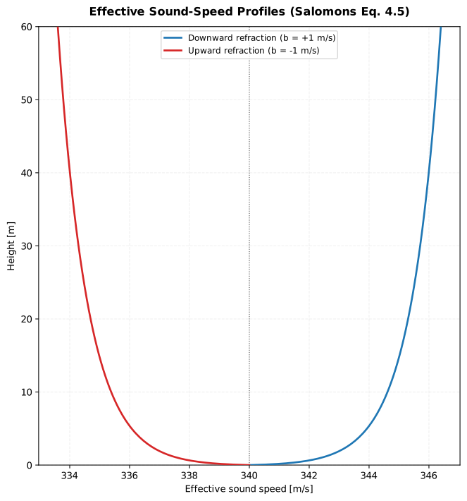

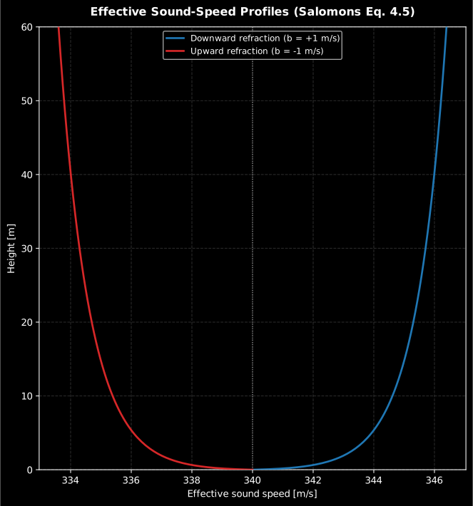
Almost all of the refraction is decided in the first few metres: over grassland the logarithmic profile spends half its 60 m change below about 1 m, which is why the source and receiver heights matter so much more outdoors than the distance between them suggests.

Show the code for this figure

import matplotlib.pyplot as plt
from phonometry import log_linear_sound_speed_profile

# The two canonical surface layers of Salomons Eq. 4.5 over grassland.
down = log_linear_sound_speed_profile(+1.0, ground_speed=340.0, max_height=60.0)
up = log_linear_sound_speed_profile(-1.0, ground_speed=340.0, max_height=60.0)
ax = down.plot(color="#1f77b4")
up.plot(ax=ax, color="#d62728")
plt.show()

2. Ray model

In geometrical acoustics a sound ray obeys Snell’s law $\cos (\gamma (z))/c(z)=\text{const}$ (Salomons Eq. 4.3). atmospheric_ray_paths integrates it with a fourth-order Runge-Kutta scheme, marching in range and reflecting specularly at the ground, and returns the curved paths, the turning points, the travel times and the number of ground reflections.

import numpy as np
from phonometry import atmospheric_ray_paths, log_linear_sound_speed_profile

profile = log_linear_sound_speed_profile(-1.0, ground_speed=340.0)
rays = atmospheric_ray_paths(profile, source_height=2.0,
                             launch_angles_deg=np.linspace(-8.0, 8.0, 17),
                             max_range=600.0)
rays.turning_points      # turning points per ray
rays.plot()              # the curved ray fan (needs matplotlib)

The page-top figure shows this upward-refracting fan opening its shadow. The favourable case is its mirror image: under downward refraction ($b=+1$) the shallow rays are bent back to the ground, bounce, and carry energy along the surface instead of losing it upward.

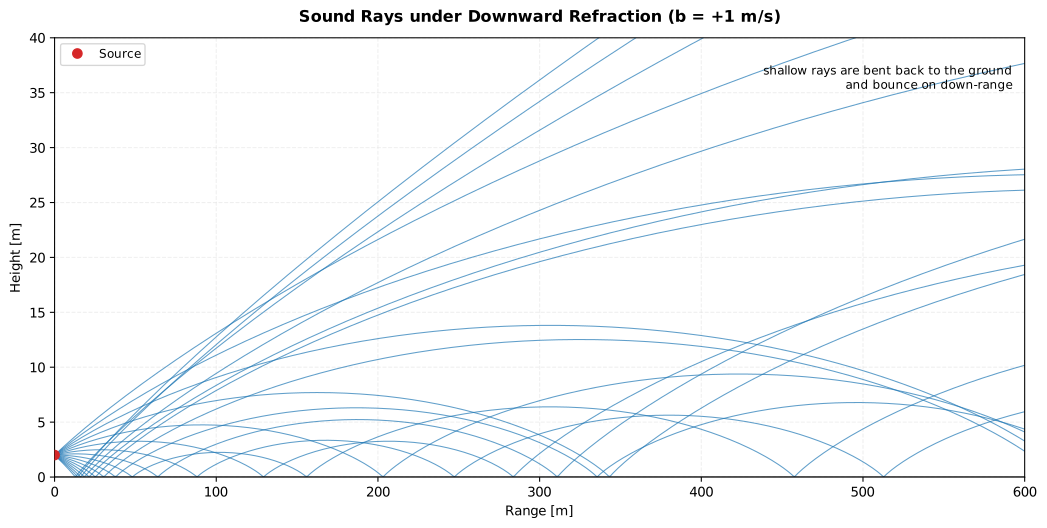
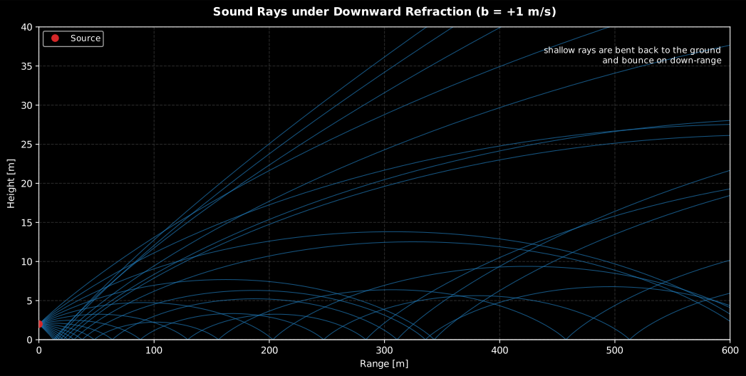
The favourable case, and the reason a downwind measurement is repeatable and an upwind one is not: the shallow rays are returned to the ground and keep hopping, so there is no shadow to fall into and no boundary whose position depends on a gradient nobody measured.

Show the code for this figure

import matplotlib.pyplot as plt
import numpy as np
from phonometry import atmospheric_ray_paths, log_linear_sound_speed_profile

# Downward refraction: the favourable-propagation mirror of the shadow case.
profile = log_linear_sound_speed_profile(+1.0, ground_speed=340.0)
rays = atmospheric_ray_paths(profile, source_height=2.0,
                             launch_angles_deg=np.linspace(-8.0, 8.0, 17),
                             max_range=600.0, n_steps=600)
rays.plot()   # shallow rays return to the ground and bounce on down-range
plt.show()

Closed-form geometry (linear gradient)

For a linear profile every ray is an exact circular arc of radius of curvature (Salomons Sec. 4.4; Attenborough Ch. 11):

$$R_c=\frac{c_0}{|g|\cos {\theta }_0},$$

exposed as ray_curvature_radius. A ray launched at angle ${\theta }_0$ in downward refraction turns at the height $R_c(1-\cos {\theta }_0)$. For an upward-refracting linear profile the ground-grazing ray bounds a region beyond which no direct or once-reflected ray arrives, at the closed-form shadow-zone distance (shadow_zone_distance):

$$x_{\text{shadow}}=\sqrt{2R_c}\left(\sqrt{h_s}+\sqrt{h_r}\right),R_c=\frac{c_0}{|g|},$$

where this second $R_c$ is the grazing (${\theta }_0=0$) special case of the expression above, since the bounding ray leaves the source horizontally.

These closed forms are the exact oracle for the ray tracer: a circle fit of a traced ray recovers $R_c$ to machine precision. They are also the cheapest answer to the question the whole page turns on — is my range long enough for refraction to matter?

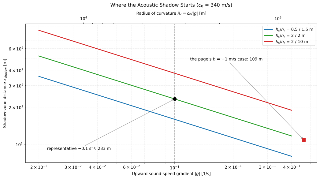
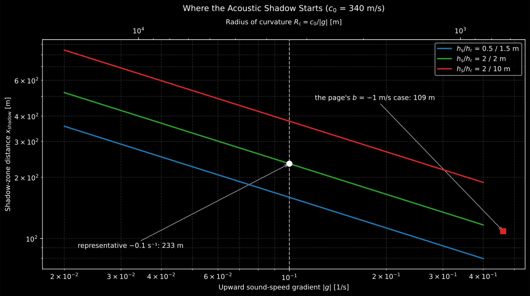
Read it as a screening test. At the representative $-0.1{\text{s}}^{-1}$ the shadow behind two 2 m stations starts at 233 m, so a 100 m measurement over a field never leaves the lit region and the homogeneous models on the neighbouring pages are the right tool. Raise the receiver and the boundary runs away fast — 2 m to 10 m pushes it from 233 m to 377 m — which is why a first-floor window hears a source a ground-floor microphone cannot.

Show the code for this figure

import matplotlib.pyplot as plt
import numpy as np

# `shadow_zone_distance` is imported by the page-top figure block.
gradients = np.geomspace(0.02, 0.4, 60)
fig, ax = plt.subplots()
for hs, hr, label in [(0.5, 1.5, "0.5 / 1.5 m"), (2.0, 2.0, "2 / 2 m"),
                      (2.0, 10.0, "2 / 10 m")]:
    ax.loglog(gradients,
              [shadow_zone_distance(-g, hs, hr, ground_speed=340.0)
               for g in gradients], label=label)
ax.set_xlabel("Upward gradient |g| [1/s]")
ax.set_ylabel("Shadow-zone distance [m]")
ax.legend()
plt.show()

3. Parabolic equation (Green’s Function PE)

The parabolic equation is the reference method for refraction and shadow zones at long range. It replaces the wave equation with a one-way (outgoing) equation valid within a limiting elevation angle, and marches it in range on a range-height grid. atmospheric_parabolic_equation implements the Green’s Function PE (GFPE, Salomons Appendix H), the atmospheric member of the same split-step Fourier family as the ocean parabolic_equation. Each range step transforms the field to the vertical-wavenumber domain, applies the free-space propagator together with the finite-impedance ground reflection $R(k_z)=(k_{z}Z-k_0)/(k_{z}Z+k_0)$ (Salomons Eq. H.28), transforms back, adds the surface-wave residue of the reflection pole (the third term of Eq. H.49) and applies the refraction phase screen $\exp (i\Delta r(k(z)-k_a))$ (Eq. H.58). The source is a Gaussian starter with its ground image (Eqs. G.64, G.76) and an absorbing layer at the top of the grid suppresses top-boundary reflections. The result is the relative sound level $\Delta L(z,r)=20{\log }_{10}(|p|R_1)$ (dB re free field) over the whole range-height plane.

from phonometry import atmospheric_parabolic_equation, log_linear_sound_speed_profile

profile = log_linear_sound_speed_profile(-1.0, ground_speed=340.0)  # upward
pe = atmospheric_parabolic_equation(400.0, profile, source_height=2.0,
                                    flow_resistivity=200e3,  # grassland
                                    max_range=600.0, max_height=40.0)
pe.level_at_height(2.0)   # relative level vs range at 2 m
pe.plot()                 # the range-height relative-level field (needs matplotlib)

Cut the field at the receiver height and the whole story of this page is one figure: with everything else identical, the sign of the gradient alone moves the 400 Hz level at 600 m by more than 30 dB.

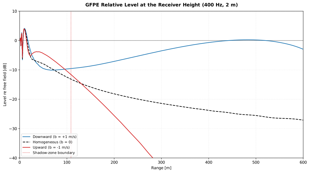
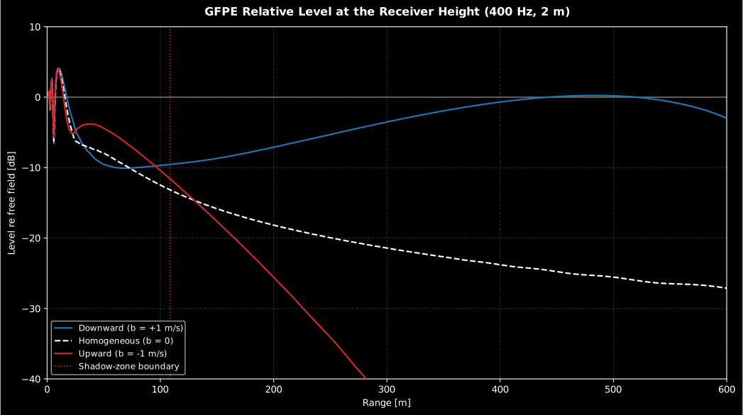
One source, one distance, one ground, three atmospheres: at 600 m the sign of the gradient alone is worth more than 30 dB. Any single-number meteorological correction — $C_{met}$ included — is an average over this spread, not a prediction of where on it a given night sits.

Show the code for this figure

import warnings

import matplotlib.pyplot as plt

from phonometry import (
    atmospheric_parabolic_equation,
    linear_sound_speed_profile,
    log_linear_sound_speed_profile,
    shadow_zone_distance,
)

cases = [
    (log_linear_sound_speed_profile(+1.0, ground_speed=340.0), "Downward (b = +1 m/s)"),
    (linear_sound_speed_profile(0.0, ground_speed=340.0), "Homogeneous (b = 0)"),
    (log_linear_sound_speed_profile(-1.0, ground_speed=340.0), "Upward (b = -1 m/s)"),
]
fig, ax = plt.subplots(figsize=(11, 6.2))
with warnings.catch_warnings():
    # The PorousAbsorberWarning: a 200 kPa.s/m2 ground runs the one-parameter
    # impedance model below its published fit range, as every outdoor ground
    # does (see "Choosing the ground impedance" in the ground-effect guide).
    warnings.simplefilter("ignore")
    for profile, label in cases:
        pe = atmospheric_parabolic_equation(400.0, profile, source_height=2.0,
                                            flow_resistivity=200e3,
                                            max_range=600.0, max_height=40.0)
        ax.plot(pe.ranges, pe.level_at_height(2.0), label=label)
# The closed-form boundary of the equivalent linear upward gradient (its
# 10 m mean), the dotted line of the figure.
up = cases[2][0]
grad = float(up.speed_at(10.0) - 340.0) / 10.0
ax.axvline(shadow_zone_distance(grad, 2.0, 2.0, ground_speed=340.0),
           color="k", ls=":", label="Shadow-zone boundary")
ax.set(xlabel="Range [m]", ylabel="Level re free field [dB]", ylim=(-40, 10))
ax.legend()
plt.show()

The ground impedance is supplied directly (impedance=, a normalized complex value in the $e^{-i\omega t}$ convention of Salomons, with $\mathrm{Im}(Z)>0$ for a passive ground), as a PorousMediumResult, or from an effective flow_resistivity via the porous models of the materials domain; the porous models work in the opposite $e^{+j\omega t}$ convention, so their impedance is conjugated internally.

The clip below runs the full wave physics through both signs of the logarithmic profile: a steady 50 Hz source 2 m over rigid ground in a 2D FDTD slice, with the library’s ray fans traced through the same $c(z)$ profiles laid over the fields. Downwind the fronts bend back and stream along the ground to the 350 m receiver; upwind they lift off the surface and the ground goes quiet beyond the ray-model shadow boundary.

A steady 50 Hz source 2 m above rigid ground in a 2D FDTD slice, downwind and upwind panels with their logarithmic effective sound-speed profiles drawn beside them. Downwind the wavefronts curve back to the ground and keep the 350 m receiver loud; upwind they lift away and an acoustic shadow opens beyond the annotated 109 m ray-model boundary, with the library ray fans overlaid and a closing spreading-compensated RMS map showing the bright ground duct against the dark shadow wedge.

Download the animation (WebM)

A steady 50 Hz source 2 m above rigid ground in a 2D FDTD slice, downwind and upwind panels with their logarithmic effective sound-speed profiles drawn beside them. Downwind the wavefronts curve back to the ground and keep the 350 m receiver loud; upwind they lift away and an acoustic shadow opens beyond the annotated 109 m ray-model boundary, with the library ray fans overlaid and a closing spreading-compensated RMS map showing the bright ground duct against the dark shadow wedge.

Download the animation (WebM)

4. Validation

The models are anchored by independent oracles, pinned numerically in the conformance report (section “Atmospheric refraction”):

• Homogeneous limit → spherical ground effect. With a zero gradient the GFPE field reproduces the exact Weyl-Van der Pol ground_effect at every range, to a few tenths of a dB over grassland on the default grid, and to the coherent +6 dB two-ray enhancement over a rigid ground.
• Exact ray geometry. For a linear profile the traced ray is a circular arc whose fitted radius matches ray_curvature_radius to machine precision.
• Reciprocity. Swapping the source and receiver heights leaves the PE level unchanged.
• Shadow zone. Over an upward-refracting profile the PE level collapses far inside the closed-form shadow distance.

The first two are worth seeing rather than trusting, because they are what licenses every other number the solver produces.

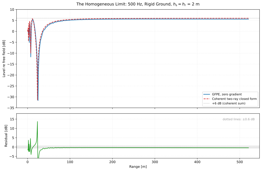
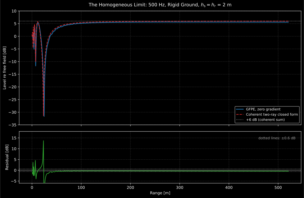
With the gradient switched off the PE has nothing left to do but reproduce the closed form, and beyond the last interference null it does: the residual stays inside 0.6 dB and both curves settle on the coherent +6 dB (PE 5.59 dB against 6.00 dB at 500 m, the pair pinned in the conformance report). Inside the null the residual reaches 17 dB, which is not a solver failure but what a −31 dB null does to any comparison expressed in decibels — the same trap as a narrowband barrier curve.

Show the code for this figure

import warnings

import matplotlib.pyplot as plt
import numpy as np

# `atmospheric_parabolic_equation` and `linear_sound_speed_profile` are
# imported by the snippets above. A rigid ground needs no porous model, so
# this case raises no warning at all.
c0, freq, zs = 343.0, 500.0, 2.0
flat = linear_sound_speed_profile(1e-12, ground_speed=c0, max_height=200.0)
with warnings.catch_warnings():
    warnings.simplefilter("ignore")
    pe = atmospheric_parabolic_equation(freq, flat, source_height=zs,
                                        impedance=1e6 + 0j, max_range=520.0,
                                        max_height=150.0)
ranges = np.asarray(pe.ranges)
solver = np.asarray(pe.level_at_height(zs))
k = 2.0 * np.pi * freq / c0
r1 = np.hypot(ranges, 0.0)
r2 = np.hypot(ranges, 2.0 * zs)
two_ray = 20.0 * np.log10(np.abs(1.0 + (r1 / r2) * np.exp(1j * k * (r2 - r1))))

fig, (top, bottom) = plt.subplots(2, 1, sharex=True)
top.plot(ranges, solver, label="GFPE, zero gradient")
top.plot(ranges, two_ray, "--", label="Coherent two-ray closed form")
top.axhline(6.0, ls=":", label="+6 dB")
top.set_ylabel("Level re free field [dB]")
top.legend()
bottom.plot(ranges, solver - two_ray)
bottom.set(xlabel="Range [m]", ylabel="Residual [dB]")
plt.show()

What this guide covers

• Covered

  The ray model (Runge-Kutta integration of Snell’s law, atmospheric_ray_paths) with the closed-form linear-profile geometry (ray_curvature_radius, shadow_zone_distance, Salomons Sec. 4.4), and the Green’s Function parabolic equation (atmospheric_parabolic_equation, Salomons Appendices G and H): the Gaussian starter, the finite-impedance ground reflection, the refraction phase screen and the absorbing top layer. Validated by the homogeneous limit against the exact spherical ground effect (a few tenths of a dB, and the +6 dB rigid-ground enhancement), exact ray geometry to machine precision, reciprocity and the shadow-zone collapse.

• Not covered

  Both models take a single effective-sound-speed profile that varies with height alone, not with range: a horizontally inhomogeneous atmosphere (a gradient that changes along the path) sits outside their range-independent formulation, described in the module as the counterpart of the “range-independent ocean solvers” it mirrors. Both also assume flat ground at $z=0$; neither takes a terrain elevation profile.

See also

• Theory: Outdoor propagation: the meteorological assumptions ISO 9613-2 makes, which is what refraction takes apart.

References

• Attenborough, K., & Van Renterghem, T. (2021). Predicting outdoor sound (2nd ed.). CRC Press. https://doi.org/10.1201/9780429470806Chapter 11 (refraction by wind and temperature gradients, ray models and shadow zones). ISBN 978-1-4987-4007-4.
• Salomons, E. M. (2001). Computational atmospheric acoustics. Kluwer Academic. https://doi.org/10.1007/978-94-010-0660-6Chapter 4 (effective sound speed, the ray model and PE examples), Appendix G (the Crank-Nicholson PE and the Gaussian starter, Eqs. G.64, G.76) and Appendix H (the Green's Function PE, the impedance reflection Eq. H.28 and the refraction factor Eq. H.58). ISBN 978-1-4020-0390-5.