Impulsive Sound Exposure Statistics (ISO 13474)

A blast, a shot or a detonation a few kilometres away is not heard at one level. The same charge fired twice from the same place reaches the same receiver ten decibels apart and more, because the wind, the temperature profile and the ground between them change from one hour to the next, and at long range they decide more of the level than the distance does. An environmental assessment of a firing range or a quarry therefore cannot ask how loud one event is. It asks how often an event is how loud.

ISO 13474:2009 answers with a statistical distribution. The weather is described as a set of replica atmospheres, each one a combination of an atmospheric-absorption class and an excess-attenuation class with its probability of occurrence; the single-event sound exposure level is computed for each; and the list of levels and probabilities is turned into a density, spread for the turbulence the replicas leave out, from which the long-term level and the level exceeded by any percentage of the events are read.

This page is that statistical core, run on the example the standard prints in its Annex A: a TOW anti-tank missile launcher heard at 3 020 m under 27 excess-attenuation classes.

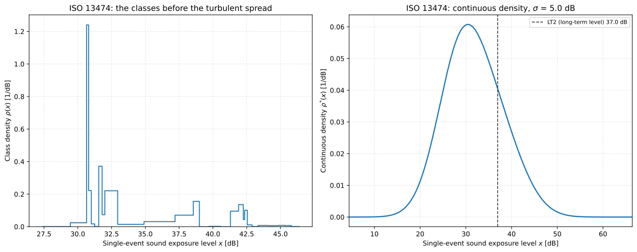
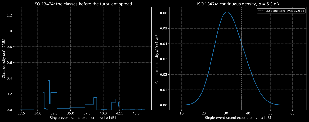
The classes of Annex A before the spread (left, Figure A.1 of the standard) and after it (right, Figure A.2), with the long-term level LT2 marked.

Each replica atmosphere gives a band sound exposure level at the receiver, the source level less the attenuation of every mechanism along the path (Equation (4)). What the statistics work on is one frequency-weighted level per replica, the energy sum over the bands of Equation (5):

The weighting is whatever the assessment uses, A or C, given as one value per band. Here it is applied to the octave-band source levels of the launcher that Annex A prints in its Table A.1, with the A-weighting at the octave centres:

from phonometry import environment

source_db = [115.0, 119.0, 134.0, 135.0, 134.0, 136.0, 133.0, 126.0]  # 31,5 Hz to 4 kHz
a_weighting_db = [-39.4, -26.2, -16.1, -8.6, -3.2, 0.0, 1.2, 1.0]
print(round(environment.frequency_weighted_sel(source_db, a_weighting_db), 1))  # 139.5

An array of shape (N_atm, N_exc, n_bands) holding the band levels of every replica returns the (N_atm, N_exc) weighted levels in one call. The probability of a replica is the product of the probabilities of its two classes, which the standard takes as independent (Equation (14)): environment.replica_probabilities(p_atm, p_exc) returns that product as the same (N_atm, N_exc) grid.

Annex A uses a single atmospheric-absorption class of probability 1, so its replicas are its 27 excess-attenuation classes. Table A.3 gives the A-weighted level of each at the receiver, and its probability by day and by night; the 07:00 to 19:00 period of the assessment is 80 % day and 20 % night:

import numpy as np

levels_db = [30.5, 31.2, 31.3, 36.1, 38.3, 38.8, 39.2,
             30.8, 31.8, 31.8, 33.7, 40.2, 41.0, 41.6, 42.2, 42.4, 42.7, 43.1,
             28.4, 30.8, 32.2, 42.3, 43.6, 44.5, 45.2, 45.5, 46.1]
day = [0.0360, 0.0053, 0.0003, 0.0731, 0.0951, 0.0634, 0.0,
       0.2037, 0.1087, 0.0184, 0.0279, 0.0001, 0.0, 0.0549, 0.0482, 0.0209, 0.0039, 0.0003,
       0.0, 0.0356, 0.2042, 0.0001, 0.0, 0.0, 0.0, 0.0, 0.0]
night = [0.0, 0.0, 0.0, 0.0664, 0.0966, 0.0962, 0.0,
         0.1151, 0.0295, 0.0, 0.0268, 0.0084, 0.0, 0.0665, 0.0445, 0.0172, 0.0033, 0.0003,
         0.0069, 0.0798, 0.2310, 0.0215, 0.0260, 0.0263, 0.0194, 0.0153, 0.0030]
probabilities = 0.8 * np.asarray(day) + 0.2 * np.asarray(night)

The expectation of the energy over the replicas is the long-term average single-event sound exposure level of Equation (7), and with the adjustment $K$ for highly impulsive sound of ISO 1996-1 inside the sum it is the rating level of Equation (8), the quantity the standard hands on to an ISO 1996-1 assessment:

print(round(environment.long_term_sel(levels_db, probabilities), 1))  # 37.0
print(round(environment.long_term_sel(levels_db, probabilities, rating_adjustment_db=12.0), 1))  # 49.0

37,0 dB is the LT1 Figure A.3 prints. It sits well above the level half the events exceed, 31,5 dB, because an energy mean is dominated by the loud minority: the downwind classes above 40 dB hold 15 % of the events and more than half of the energy.

To turn the list into a distribution, Equation (10) sorts the levels, and each becomes a class whose boundaries lie half-way between it and its neighbours (Equation (11)); the two outer boundaries mirror the nearest inner one about the end level (Equations (12) and (13)). The probability of a class spread evenly over its width is its density (Equation (15)):

dist = environment.sel_distribution(levels_db, probabilities, sigma_db=5.0, subclasses=10)
print(dist.levels_db[:4])                         # [28.4 30.5 30.8 30.8]
print(dist.lower_bounds_db[:4].round(2))          # [27.35 29.45 30.65 30.8 ]
print([round(float(r), 4) for r in dist.class_densities_per_db[:4]])  # [0.0007, 0.024, 1.2399, 0.2222]
print(dist.replicas[2], dist.replicas[3])         # (7,) (19,)

That is Table A.4, and every one of its 27 rows comes out digit for digit. Two things in it are worth seeing. The class densities are the full-precision probabilities over the widths, not the rounded column printed beside them: 0,1860 over 0,15 dB would print 1,2400, and the table prints 1,2399. And two pairs of classes share a level, 30,8 dB (Table A.3 rows 8 and 20) and 31,8 dB (rows 9 and 10). Equation (11) puts their common boundary at that level and each keeps its half on its own side, so the table keeps both, and replicas says which input each came from. The standard names the case of three consecutive equal levels, whose middle class has no width, and for it tells you to combine classes of the same level; a pair at either end of the list has the same problem through Equation (12) or (13), which the standard does not mention and the library treats the same way. sel_distribution combines exactly those runs and leaves every other pair as Annex A does.

The replicas describe the average state of the atmosphere, not its random perturbations, and field measurements show a spread of the level about each replica that the standard models as a normal distribution with a standard deviation of typically 5 dB. The convolution is carried out in two steps. Each class is split into $N_{\mathrm{sub}}$ equal subclasses centred at ${\mu }_{m,j}$ (Equations (17) and (18)), ten in Annex A; each subclass is then replaced by a Gaussian carrying its probability (Equation (21)).

The Gaussian is not centred on the subclass. A level is a logarithm of an energy, and a symmetric spread of the level raises the mean energy, so each Gaussian is centred $\Delta \mu$ below the subclass to keep its energetic mean where the subclass was (Equation (22)):

print(round(environment.turbulence_level_shift(5.0), 3))   # 2.878
print(round(dist.level_shift_db, 3))                       # 2.878

Annex A says the shift of its example was 1,04 dB. That is Equation (22) at a standard deviation of 3 dB, not at the 5 dB of the same paragraph, and the rest of the annex was computed with 2,878 dB: with 1,04 dB every level of the distribution would move up by 1,84 dB and the long-term level of the next section would read 38,8 dB, not 37,0 dB. The errata register has the entry. The library evaluates the integral in closed form, so the shift is not a parameter.

The spread density ${\rho }^{\ast }(x)$ is continuous, and everything is read from it. The probability that an event exceeds $x$ is its upper tail (Equation (24)), and the $n$-percent exceedance level is the level exceeded with probability $n/100$ (Equation (25)):

print(dist.exceedance_level([95.0, 50.0, 10.0, 5.0, 1.0]).round(1))  # [21.6 31.5 40.5 43.  47.5]
print(round(dist.exceedance(37.0), 3))                                 # 0.214
print(round(dist.long_term_level_db, 2), round(dist.distribution_long_term_level_db, 2))  # 37.01 36.96

The long-term level taken a second time, over the continuous density (Equation (A.4), LT2), differs from LT1 only by where each class’s energy sits inside its width, and both print 37,0 dB, which is the agreement the annex offers as its check. The probability that one event exceeds the long-term level is 21 %: one event in five is louder than the level that stands for all of them.

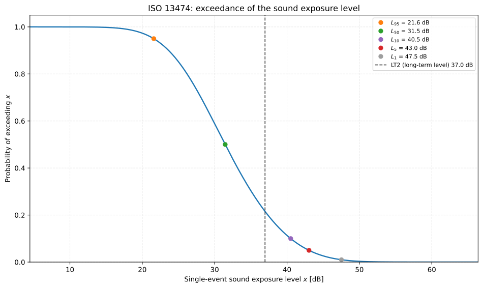
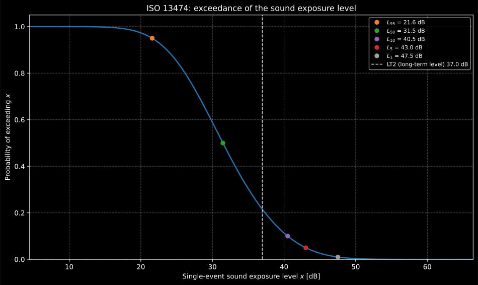
The exceedance curve of the Annex A example with the five percentiles Figure A.3 lists, as Equation (25) gives them, from dist.plot(view="exceedance").

Figure A.3 prints those five levels as 21,7; 31,5; 40,6; 43,2 and 48,0 dB. $L_{50}$ agrees; the other four are 0,1 dB to 0,5 dB higher in print, the more so the rarer the level, and the annex does not say how it computed them. They are consistent with a curve accumulated from 15 dB, where the drawn curve begins (the axis starts at 10 dB), rather than from minus infinity, when that curve is fed the 07:00 to 19:00 column of Table A.3 as printed: all five then come out to the printed digit. Fed the full-precision probabilities that reproduce Table A.4, as dist above is, the same reading gives 48,05 dB for $L_1$, which would print 48,1 dB, so it stays a hypothesis. The errata register has the entry, and the library evaluates Equation (24) as written.

import matplotlib.pyplot as plt

fig, (ax_classes, ax_density) = plt.subplots(1, 2, figsize=(13.5, 5.4))
dist.plot(ax_classes, view="classes")   # Figure A.1: the step density
dist.plot(ax_density)                   # Figure A.2: the spread density
dist.plot(view="exceedance")            # Figure A.3: the exceedance curve
plt.show()

• Covered

  ISO 13474:2009, the statistical core: the frequency-weighted single-event level of Equation (5) from band levels, for any weighting; the probability of each replica atmosphere as the product of its two class probabilities (Equation (14)); the long-term average single-event level of Equation (7) and the rating level with $K$ of Equation (8); the ordered classes, their boundaries and densities of Equations (10) to (16), with the combination of equal levels where a class would have no width; the subclasses and the Gaussian spread of Equations (17) to (23), with the shift of Equation (22) in closed form; the exceedance probability and the $n$-percent exceedance level of Equations (24) and (25); and the long-term level over the continuous density of Equation (A.4). Table A.4 of Annex A is reproduced digit for digit from Table A.3, and LT1, LT2 and $L_{50}$ match Figure A.3.

• Not covered

  The levels of the replica atmospheres are an input. The propagation that produces them is not implemented here: the attenuation terms of clause 6 (divergence, atmospheric absorption, screening, terrain and the excess attenuation from a parabolic-equation model), the classification of the atmosphere of clause 7, the probability of each class from meteorological data of clause 8, the ground impedances of Table 1, and the source descriptors of clause 9. The equivalent level over an assessment period of Equation (9) is not given a function of its own, and the uncertainty budget of Annex B is not modelled. The atmospheric refraction guide below computes the excess attenuation of one sound speed profile, which is where a replica level would start.

References

Section titled “References”- International Organization for Standardization. (2009). Acoustics — Framework for calculating a distribution of sound exposure levels for impulsive sound events for the purposes of environmental noise assessment (ISO 13474:2009). The implemented statistical core: the frequency-weighted level of Equation (5), the long-term average and rating level of Equations (7) and (8), the ordered classes of Equations (10) to (16), the subclasses and Gaussian spread of Equations (17) to (23), the exceedance of Equations (24) and (25), and the long-term level of Equation (A.4). Read from BS ISO 13474:2009, the UK implementation of the standard, whose pages carry the ISO 13474:2009(E) text; its Annex A is the worked example this page runs.
- International Organization for Standardization. (2016). Acoustics — Description, measurement and assessment of environmental noise — Part 1: Basic quantities and assessment procedures (ISO 1996-1:2016). Where the rating level adjustment K for highly impulsive sound comes from, and the assessment the long-term rating level of ISO 13474 is offered to.