A road surface makes no noise of its own, yet the same traffic can be up to 15 dB louder on one surface than on another (the Introduction of ISO 11819-1 gives that range). Texture and porosity both change how much noise the tyres make, and porosity also changes how it propagates close to the ground. ISO 11819-1 is the method that measures this, and ranks surfaces by it. It does so without choosing any vehicles: it measures the traffic that happens to use the road, one isolated vehicle at a time, and lets statistics take the vehicles out.
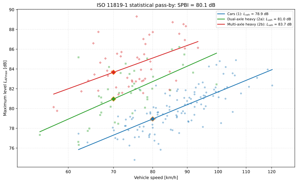
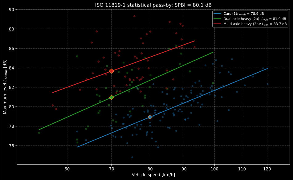
One site, three categories of vehicle, three straight lines in the logarithm of speed, and the three points on them that the index is made of.
1. What is measured, and on which vehicles
Section titled “1. What is measured, and on which vehicles”Every vehicle measured is put in one of three categories (3.4): cars (1), dual-axle heavy vehicles (2a), trucks, buses and coaches with two axles and more than four wheels, and multi-axle heavy vehicles (2b), those with more than two axles. Vans, cars with trailers and motorcycles are not used, because they add nothing about the surface (clause 4), and a vehicle that cannot be classified without doubt is discarded (7.1).
The road is put in one of three speed categories (3.3), by the average speed of its traffic: low, 45 km/h to 64 km/h, usually urban; medium, 65 km/h to 99 km/h, suburban roads and rural highways; high, cars at 100 km/h or more, usually motorways. Each speed category fixes a reference speed per vehicle category, the speed every level is brought to, and the share each category is given in the index (Table 1).
| Vehicle category | Low: speed | Low: | Medium: speed | Medium: | High: speed | High: |
|---|---|---|---|---|---|---|
| Cars (1) | 50 km/h | 0,900 | 80 km/h | 0,800 | 110 km/h | 0,700 |
| Dual-axle heavy (2a) | 50 km/h | 0,075 | 70 km/h | 0,100 | 85 km/h | 0,075 |
| Multi-axle heavy (2b) | 50 km/h | 0,025 | 70 km/h | 0,100 | 85 km/h | 0,225 |
The table is environment.SPB_REFERENCE_SPEEDS_KMH and
environment.SPB_WEIGHTING_FACTORS, keyed by road speed category and then by
vehicle category.
How the measurement goes
Section titled “How the measurement goes”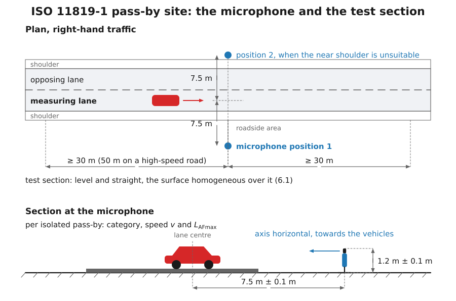
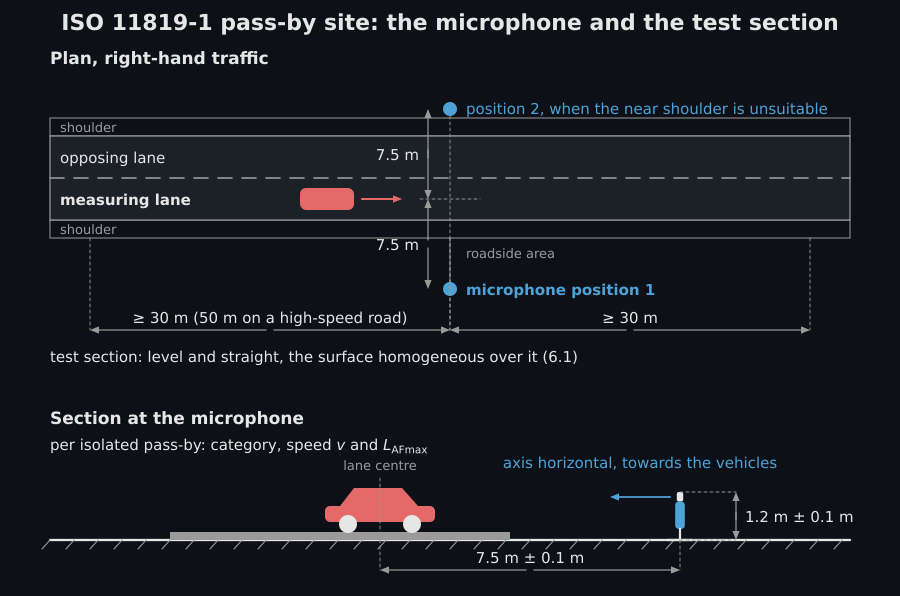
One microphone beside one lane of real traffic: every vehicle that passes on its own gives one point, its category, its speed and its maximum level.
| Requirement | Value | Clause |
|---|---|---|
| Microphone | 7,5 m ± 0,1 m from the centre of the test lane, 1,2 m ± 0,1 m above it, axis horizontal and towards the vehicles | 8.1 |
| Level | Maximum A-weighted sound pressure level, time weighting F, of each pass-by; type 1 meter, windscreen, calibration checked before and after, a drift over 0,5 dB invalidates the series | 5.1, 5.3, 8.2 |
| Speed | At the moment the vehicle midpoint passes the microphone, standard uncertainty under 3 %; radar readings corrected for the angle; no devices on the road surface | 5.4, 8.4 |
| Which pass-bys | The level at least 6 dB lower just before and just after the vehicle; no overtaking or opposing traffic at the peak; constant speed; normal lateral position; no rattles, faulty exhausts or sirens | 7.2 |
| How many | At least 100 cars, 30 dual-axle, 30 multi-axle and 80 heavy vehicles together, for surface classification | 7.3 |
| The site | Level and straight over 30 m each side of the microphone (50 m on a high-speed road); reflections at least 10 dB under the direct sound, about 25 m clear of reflecting objects; at least half the ground to the microphone acoustically like the road | 6.1, 6.3, 6.5 |
| Weather | Wind at the microphone at most 5 m/s; air 5 °C to 30 °C; road surface 5 °C to 50 °C; the surface dry, pores included | 11 |
| Background | At least 10 dB under the quietest pass-by kept | 12 |
2. The vehicle sound level
Section titled “2. The vehicle sound level”For each vehicle category the pass-bys are fitted by least squares with a straight line in the logarithm of speed (9.1),
and the line is read at the reference speed of Table 1. That ordinate is the vehicle sound level of the category (9.2): what a typical vehicle of it emits at that speed on this surface. The logarithm of speed is the axis the clause fits in, which is why the figure draws speed on a logarithmic scale, where each cloud is a band and its fit a straight line.
import numpy as npfrom phonometry import environment
rng = np.random.default_rng(11819)# A medium-speed site: per category, the number of pass-bys, the mean speed# (km/h), the spread of lg v, and the line and scatter (dB) they are drawn about.site = {    "1": (120, 88.0, 0.055, 16.6, 32.6, 1.4),    "2a": (40, 76.0, 0.050, 46.5, 18.8, 2.0),    "2b": (50, 74.0, 0.045, 34.5, 26.7, 2.0),}categories, speeds, levels = [], [], []for category, (n, mean_kmh, spread, a, b, scatter) in site.items():    lg_v = np.log10(mean_kmh) + spread * rng.standard_normal(n)    categories += [category] * n    speeds += (10.0**lg_v).tolist()    levels += (a + b * lg_v + scatter * rng.standard_normal(n)).tolist()
result = environment.statistical_pass_by(    categories, speeds, levels, road_speed_category="medium")print(dict(result.reported_vehicle_sound_levels_db))# {'1': 78.9, '2a': 81.0, '2b': 83.7}   dB, at 80, 70 and 70 km/hcars = result.regressions["1"]print(round(cars.slope_db_per_decade, 2), round(cars.correlation, 2))# 28.22 0.75print(round(cars.residual_standard_deviation_db, 2), round(cars.mean_speed_kmh, 1))# 1.4 86.9
Each regression carries what clause 13 asks to be reported about it (item 29):
the slope and the intercept, the standard deviation of the speeds and of the
residuals about the line, and the mean speed. The mean speed is
, the mean of the variable the line is fitted in turned
back into km/h, which is also what Annex E prints under “Value converted from
the logarithm of speed”. The standard deviation of the speeds is given in the
same variable, lg_speed_standard_deviation, because that is the one the line
is fitted in and the one 9.3 is judged in.
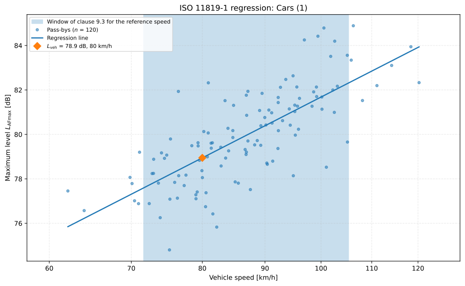
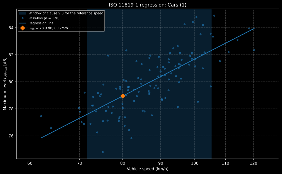
The line is only read at a speed the measured traffic actually covers: the shaded window is where 9.3 allows the reference speed to lie.
Show the code for these figures
import matplotlib.pyplot as plt
result.plot()                    # the three categories and the indexresult.regressions["1"].plot()   # one category, its window and L_vehplt.show()
Two conditions, judged and not enforced. A regression is only a fair way to
move levels to a reference speed if the traffic was near that speed. Clause 9.3
therefore asks the reference speed to lie within one standard deviation of the
measured mean speed for heavy vehicles and within one and a half for cars. The
library judges it in the variable of the fit, ,
reports the window in km/h as speed_window_kmh and the verdict as
reference_speed_in_window. Clause 7.3 asks for 100 cars, 30 vehicles of each
heavy category and 80 heavy vehicles in all when the purpose is to classify the
surface. Both are kept on the result and, when either fails, emitted as
StatisticalPassByWarning rather than raised: a before-and-after study of one
site (6.6) is still a pass-by measurement, just not a classification.
3. The index
Section titled “3. The index”The three vehicle sound levels are added on an energy basis into one number, the Statistical Pass-By Index (9.5):
The weights are the assumed proportions of the three categories, and the speed ratios are there because the index stands for the energy of a flow: a lorry at 70 km/h is heard for longer than a car at 80 km/h, in proportion to the ratio of the two speeds. The index is therefore close to the mean of the three levels but is not an equivalent level of any real traffic (9.5 NOTE); it compares surfaces under a standard mix and does not predict what a street will measure.
print(round(result.index_db, 3), result.reported_index_db)# 80.14 80.1 dBThe index adds the vehicle sound levels as 9.2 reports them, to one decimal:
9.5 defines , and as the vehicle sound levels “according
to 9.2”, and 9.2 has every level “calculated to two decimal places and rounded
to one decimal place”. The regressions are carried at full precision and each
level is rounded once, half up (reported_vehicle_sound_levels_db, 78,9, 81,0
and 83,7 dB here); index_db is the index of those three levels, rounded once
more when it is reported. The index of the unrounded levels stays on the result
as full_precision_index_db, 80,153 dB for this site.
Table 1 is the standard mix. 9.5 recognises that national mixes differ and
allows other factors, provided they are stated; weighting_factors takes them
and refuses factors that are not proportions (negative, or not adding up to 1).
Because every has to be reported, anyone can recompute the index
for a mix of their own from a report, with statistical_pass_by_index.
4. Against a reference surface
Section titled “4. Against a reference surface”In many cases the index is used as a difference from a reference surface (9.5, clause 10), and clause 10 offers four: a real dense asphalt concrete of 11 mm to 16 mm chippings, at least a year old, with a macrotexture depth of 0,50 mm to 1,00 mm measured by ISO 10844 or ISO 13473-1 and its air voids or absorption within the requirements of ISO 10844 (10.1, the general case); a normalized reference case (10.2), a fictitious surface whose levels are set by convention, usually the average of many such surfaces; the same general surface at the same age as the one tested (10.3); and any surface the tester chooses (10.4), which only compares the surfaces measured together.
Annex D shows how a normalized case is built, from seven dense bituminous
surfaces for the medium speed range (four asphalt concrete and three stone
mastic asphalt), and prints their average. normalized_reference_levels
averages any set of surfaces the same way, and the Annex D rows and their
average are published as SPB_ANNEX_D_SURFACES_DB and
SPB_NORMALIZED_REFERENCE_DB. Hand the reference to statistical_pass_by as an
index, used as given, or as its three levels, whose index is computed from
them to one decimal with the same weighting factors:
result = environment.statistical_pass_by( categories, speeds, levels, road_speed_category="medium", reference_db=environment.SPB_NORMALIZED_REFERENCE_DB,)print(round(result.reference_index_db, 2), round(result.difference_db, 2))# 78.92 1.22 dB: this surface is 1.2 dB louder than the Annex D referenceThe Annex D surfaces are an example of how to build a reference, not a reference the standard sets: the annex asks that the surfaces behind every version of a reference be kept on record, so that a difference quoted against it can be traced.
5. Temperature
Section titled “5. Temperature”Tyre-road noise depends on temperature, and 9.4 asks for the vehicle sound
levels to be corrected to 20 °C air, but says in the same clause that “a
suitable method is at present under consideration” and makes only the
uncorrected levels mandatory. No correction is invented here. Levels corrected
by a method of your choosing go in as corrected_vehicle_sound_levels_db, and
the index is computed for them too, from the levels rounded to one decimal
(reported_corrected_vehicle_sound_levels_db, corrected_index_db). Clause 13
lists the corrected levels and index as optional report items (26 and 28)
beside the mandatory uncorrected ones (25 and 27). Where the air
temperature was taken at every pass-by, 9.4 prefers to correct each measured
level instead; correct max_levels_db and call the method again.
6. How precise it is
Section titled “6. How precise it is”Table 2 gives the random error pre-normative research found: individual
vehicles scatter about by 1,5 dB for cars and 2,0 dB for heavy
vehicles, which leaves a 95 % confidence interval of 0,3 dB and 0,7 dB on the
vehicle sound level for 100 cars and 40 heavy vehicles of each type
(SPB_VEHICLE_STANDARD_DEVIATIONS_DB, SPB_CONFIDENCE_INTERVALS_DB). They
describe the medium and high speed categories; the low one is sensitive to
acceleration and should be treated with caution (9.6).
A measurement also carries its own interval. confidence_interval_db is the
95 % interval of the fitted line at the reference speed, from the Student
distribution with degrees of freedom, which widens as the reference
speed moves away from the mean speed. The standard says the random error of the
index is “a combination of these errors according to the chosen weighting
factors” and gives no formula; index_confidence_interval_db combines the
three intervals through the sensitivity of the index to each level,
, taking the three categories as
independent.
print([round(r.confidence_interval_db, 2) for r in result.regressions.values()])# [0.3, 0.71, 0.69] dB, cars and the two heavy categoriesprint(round(result.index_confidence_interval_db, 2))# 0.27 dBBeyond the random error, 9.6 lists the systematic ones: about ±1 dB for a precision instrument system, and 0,3 dB to 0,8 dB for the variation of the vehicle fleet within a country. Annex C adds that results should not be expected to stay valid for more than about five years, as vehicles and tyres change.
7. The example of Annex E, and the rounding it uses
Section titled “7. The example of Annex E, and the rounding it uses”Annex E is a complete test report for a Swedish single surface dressing on a medium-speed road. It prints each category’s regression line, the vehicle sound levels 78,5, 81,1 and 83,8 dB, the index 79,9 dB, the index of the temperature-corrected levels (78,8, 81,1 and 83,8 dB) 80,1 dB, and a temperature-corrected difference of 2,8 dB, 80,1 dB less the 77,3 dB of its reference surface. The conformance suite reproduces every one of these numbers, the uncorrected index from pass-bys placed on the printed lines.
Which levels the index adds is settled by the clauses, not left to the example. 9.2 ends “All levels shall be calculated to two decimal places and rounded to one decimal place”, and 9.5 defines the levels of its formula as “the Vehicle Sound Levels for vehicle categories 1, 2a and 2b according to 9.2”: the index adds the levels as 9.2 reports them, to one decimal. That is also what lets anyone recompute it from a report, which 7.4 (“The sound levels Lveh and the SPBI calculated from them”) and 9.5 (the mandatory reporting of every “allows such SPBI calculations to be made”) rely on. The library follows that chain, and so does the example: its printed levels give 79,946 dB, the 79,9 it prints.
import math
printed = {"1": 78.5, "2a": 81.1, "2b": 83.8}print(round(environment.statistical_pass_by_index(printed, road_speed_category="medium"), 3))# 79.946   the levels of 9.2, to one decimal: Annex E prints 79.9lines = {"1": (16.6, 32.55, 80.0), "2a": (46.5, 18.76, 70.0), "2b": (34.5, 26.74, 70.0)}unrounded = {k: a + b * math.log10(v) for k, (a, b, v) in lines.items()}print(round(environment.statistical_pass_by_index(unrounded, road_speed_category="medium"), 3))# 79.985   the same levels left unrounded: it would print 80.0
Carried unrounded from the printed lines, the levels are 78,546, 81,114 and
83,838 dB and their index 79,985 dB, which would print 80,0; the result
keeps that chain as full_precision_index_db. The lines alone cannot tell the
two chains apart, because their intercepts are printed to one decimal and their
slopes to two: over every line that agrees with the intercept, slope, mean
level, mean speed and vehicle sound level Annex E prints, to their last digit,
the unrounded index runs from 79,948 dB to 79,996 dB. What the page does show
is that the index is rounded once: 79,946 dB taken first to two decimals,
79,95, and then to one would print 80,0 as well. The two chains never differ by
more than 0,05 dB, the most a level moves when it is rounded, which is below any
precision the method claims but can move the last printed digit. The
conformance row that pins 79,9 dB reads index_db of the run from pass-bys.
Two more things about Annex E are worth knowing before it is used as a check. Its reference index of 77,3 dB is described as a normalized reference case of seven surfaces, three stone mastic asphalt and four asphalt concrete, which is the composition of Annex D; but the Annex D levels give an index of 78,92 dB with the same weights, not 77,3, and the reference box gives a maximum chipping size of 12 mm to 16 mm where Annex D lists a surface with 11 mm chippings. The standard does not say the two are the same database, so the library treats 77,3 dB as the input it is printed as. And its speed spreads (13,3, 7,5 and 6,4 km/h) do not fit the slopes, correlations and level spreads printed beside them; the errata registry has the arithmetic. The vehicle sound levels depend on neither.
What this guide covers
Section titled “What this guide covers”Covered
The computation of ISO 11819-1:1997 from a list of measured pass-bys:
pass_by_regression(9.1, 9.2 and the 9.3 window),statistical_pass_by(the three categories, the 7.3 counts, the index of 9.5 from the levels of 9.2 to one decimal, temperature-corrected levels as an input, and the difference from a reference surface given as an index or as levels),statistical_pass_by_indexfor levels already reported, andnormalized_reference_levelsfor a reference built as in 10.2 and Annex D. Tables 1 and 2, the 7.3 counts and the 9.3 factors are published as read-only tables, and both results draw themselves with.plot().Not covered
The measurement itself: telling a vehicle’s category, screening pass-bys for the 6 dB dips of 7.2, the site and weather requirements of clauses 6, 11 and 12, which are documented above as conditions and are the tester’s. A temperature correction, which the standard does not give. The Close-Proximity method of ISO 11819-2, which works with reference tyres rather than with the traffic (Annex C, NOTE 3). Later editions of ISO 11819-1 were not consulted; this page implements the 1997 text.
References
Section titled “References”- International Organization for Standardization. (1994). Acoustics — Test surface for road vehicle noise measurement (ISO 10844:1994). One of the two methods 10.1 accepts for the macrotexture depth of the general reference surface, and the air-voids or absorption requirement that surface has to meet.
- International Organization for Standardization. (1997). Acoustics — Characterization of pavement texture by use of surface profiles — Part 1: Determination of Mean Profile Depth (ISO 13473-1:1997). The macrotexture depth that 10.1 bounds between 0,50 mm and 1,00 mm, measured on the reference surface.
- International Organization for Standardization. (1997). Acoustics — Measurement of the influence of road surfaces on traffic noise — Part 1: Statistical Pass-By method (ISO 11819-1:1997). The implemented edition: the vehicle and road speed categories of clause 3, the minimum counts of 7.3, the regression of 9.1, the vehicle sound level and Table 1 of 9.2, the speed window of 9.3, the index of 9.5, the random errors of Table 2, the reference cases of clause 10 and the examples of Annexes D and E. Read from BS EN ISO 11819-1:2001, which is identical to it.