CNOSSOS-EU railway source emission

A road is one source line 5 cm above the pavement. A railway track is two, one at the axles and one at the roof, because a train radiates from places that are four metres apart and shield each other differently. Section 2.3 of Annex II of Directive 2002/49/EC, as replaced by the CNOSSOS-EU methods, builds both of them from a roughness spectrum, a handful of transfer functions and the traffic flow.

This guide covers the railway source, section 2.3 of Annex II with the coefficient database of Appendix G. The road source (2.2, Appendix F) and the CNOSSOS-EU propagation model (2.5) are separate.

1. Which text is implemented

Annex II is a moving target, and on the railway side the layering is worse than on the road side: the corrigendum replaced the whole of Appendix G, and the 2021 amendment then replaced five of its seven tables again and rewrote three pieces of the method.

Instrument	What it does to the railway source
Commission Directive (EU) 2015/996	Replaces the whole of Annex II. Supplies formulae 2.3.1 to 2.3.18 and Tables G-1 to G-7.
Corrigendum of OJ L 5, 10.1.2018	Replaces the whole of Appendix G (dropping its Min/Max validity columns and adding the descriptor codes to the column headers) and corrects the roughness conversion f = v/lambda, where the published text says the speed is in km/h. It is in metres per second: read literally, the printed formula is wrong by a factor 3,6.
Commission Delegated Directive (EU) 2021/1226	Replaces Tables G-1b, G-2, G-3a, G-4 and G-7 in their entirety; substitutes a new curve-squeal rule; makes bridge noise a separate source built on a transfer function instead of a constant; rewrites the vertical directivity of source A; corrects three band labels and one pair of values in Table G-5.

The library implements the consolidated result, and every shipped table records in its comment which instrument it came from. Three of the 2021 changes are behavioural, not cosmetic, so a comparison with a pre-2021 study has to account for them: the rail roughness of an average network is now much higher at long wavelengths, the bridge correction has a spectrum instead of a flat 1 dB or 4 dB, and the vertical directivity is identically zero below the horizon where the old form gave a positive correction.

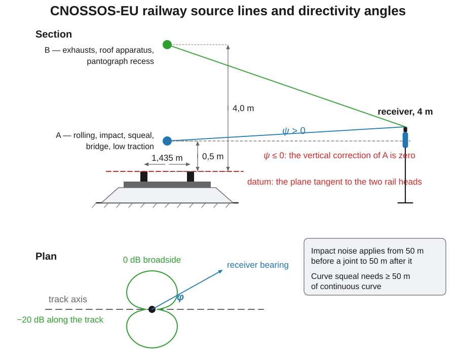
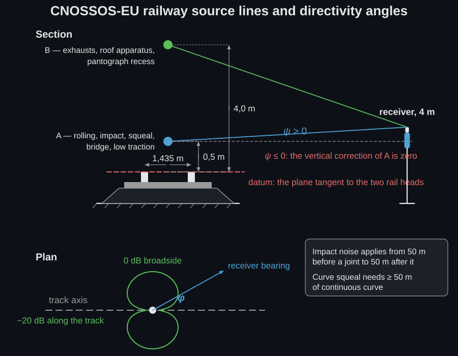
2. Two source lines, and what sits on each

The method places two incoherent source lines at the centre of the track, referred to the plane tangent to the two upper rail surfaces:

Height	Index	Physical sources allocated to it
0,5 m (source A)	$h=1$	Rolling noise (rail, wheel and freight superstructure), impact noise, curve squeal, bridge noise, and the traction and aerodynamic components that sit low: gears, motors, shrouds and screens.
4,0 m (source B)	$h=2$	The traction and aerodynamic components that sit high: diesel exhausts, roof apparatus, the pantograph recess.

Nothing in the method decides the traction split for you. Table G-5 tabulates the traction sound power separately for the two heights, so the split is read from the database rather than assumed; the Directive only adds that where a real component sits between the two model heights, its energy is distributed proportionately over them.

From a real line to the descriptors

The descriptors of Tables [2.3.a] and [2.3.b] are the interface between a national rolling-stock and track register and the shipped tables: each digit of the code selects one of them. A vehicle carries four digits and a track six.

Vehicle digit	What it selects	Codes	Library
1	Vehicle type	h high speed (> 200 km/h), m self-propelled passenger coach, p hauled passenger coach, c city tram or light metro, d diesel loco, e electric loco, a generic freight, o other	Chooses the TractionVehicle row of Table G-5 and whether the freight superstructure term applies
2	Number of axles per vehicle	the actual number	RollingStock(axles=...), the $10{\log }_{10}{N}_a$ of (2.3.8)
3	Brake type	c cast-iron block, k composite or sinter metal block, n non-tread braked (disc, drum, magnetic)	BrakeType.CAST_IRON / .COMPOSITE / .NON_TREAD → the wheel roughness of G-1a
4	Wheel measure	n none, d dampers, s screens, o other	Not a table selector in Appendix G

Track digit	What it selects	Codes	Library
1	Track base	B ballast, S slab, L ballasted bridge, N non-ballasted bridge, T embedded, O other	With digit 3, the TrackTransferClass of G-3a; L/N also switch on the bridge source of section 8
2	Railhead roughness	E well maintained and very smooth, M normally maintained, N not well maintained, B not maintained and bad	RailRoughnessClass.WELL_MAINTAINED / .NORMAL / .NOT_WELL_MAINTAINED / .BAD → G-1b
3	Rail pad type	S soft (150-250 MN/m), M medium (250-800), H stiff (800-1 000)	The second half of the TrackTransferClass label: MONOBLOCK_MEDIUM is “M/M”
4	Additional measures	N none, D rail damper, B low barrier, A absorber plate on slab, E embedded rail, O other	Outside the emission model
5	Rail joints	N none, S a single joint or switch, D two per 100 m, M more than two per 100 m	The joint density $n_l$ of (2.3.12)
6	Curvature	N straight, L 1 000-500 m, M below 500 and above 300 m, H below 300 m	The radius passed to curve_squeal_excess

Two selectors have no descriptor digit at all and have to come from the vehicle data sheet: the wheel diameter (WheelDiameter, which picks the wheel transfer function of G-3b) and the contact filter (ContactFilter, an axle load in kN paired with that diameter, Table G-2). The snippets on this page name the enum members directly for exactly that reason.

When the register does not answer, the method itself runs out: roughness classes N and B carry no spectrum in Appendix G and must be supplied by the Member State, and the same is true of a track system that matches no G-3a row — there is no default and no interpolation, so the honest step is to declare the substituted spectrum alongside the result.

For each 1/3-octave band the flow equation turns a single-vehicle sound power into a power per metre of line (2.3.2):

$$L_{W,\mathrm{eq},\mathrm{line},i}^{\prime }(\psi ,\phi )=L_{W,0,\mathrm{dir},i}(\psi ,\phi )+10{\log }_{10}\left(\frac{Q}{1000v}\right),$$

or, for a stationary vehicle, the same directional power referred to the idling time over the reference period (2.3.4):

$$L_{W,\mathrm{eq},\mathrm{line},i}^{\prime }(\psi ,\phi )=L_{W,0,\mathrm{dir},i}(\psi ,\phi )+10{\log }_{10}\left(\frac{T_{\mathrm{idle}}}{T_{\mathrm{ref}}L}\right).$$

The second replaces the first; it does not add to it. $Q$ is in vehicles per hour, $v$ in km/h, $L$ the length of the track section in metres, and $T_{\mathrm{idle}}$ and $T_{\mathrm{ref}}$ share whatever unit of time they are given in. Note the unit: the flow term uses km/h, while the roughness conversion two sections down uses m/s. Both are correct, and mixing them up is the single most expensive mistake available in this model.

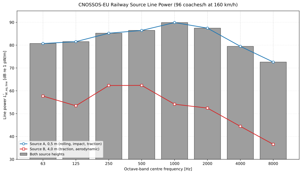
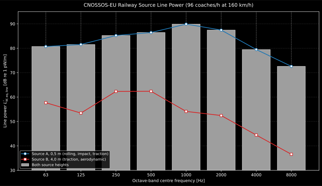
At 160 km/h the track is source A almost everywhere: the 4,0 m line only carries the traction noise of the unit, some twenty-five decibels below. It is above 200 km/h, when aerodynamic noise appears at the pantograph, that source B starts to matter.

Show the code for this figure

import matplotlib.pyplot as plt
from phonometry import (
    BrakeType, ContactFilter, RailRoughnessClass, RailwayTrack, RailwayVehicle,
    RollingStock, TrackTransferClass, TractionVehicle, WheelDiameter,
    aerodynamic_sound_power, contact_filter, impact_roughness_single,
    rail_roughness, railway_source_power, track_transfer, traction_sound_power,
    wheel_roughness, wheel_transfer,
)

stock = RollingStock(
    axles=4,
    wheel_roughness=wheel_roughness(BrakeType.NON_TREAD),
    contact_filter=contact_filter(ContactFilter.LOAD_50_DIAMETER_920),
    wheel_transfer=wheel_transfer(WheelDiameter.MM_920),
    traction=traction_sound_power(TractionVehicle.ELECTRIC_MULTIPLE_UNIT),
    aerodynamic=aerodynamic_sound_power(),
)
track = RailwayTrack(
    rail_roughness=rail_roughness(RailRoughnessClass.NORMAL),
    track_transfer=track_transfer(TrackTransferClass.MONOBLOCK_MEDIUM),
    impact_roughness=impact_roughness_single(),
)
result = railway_source_power(
    RailwayVehicle(stock, flow_rate=96.0, speed=160.0), track, phi=90.0, psi=10.0,
)
result.plot()
plt.show()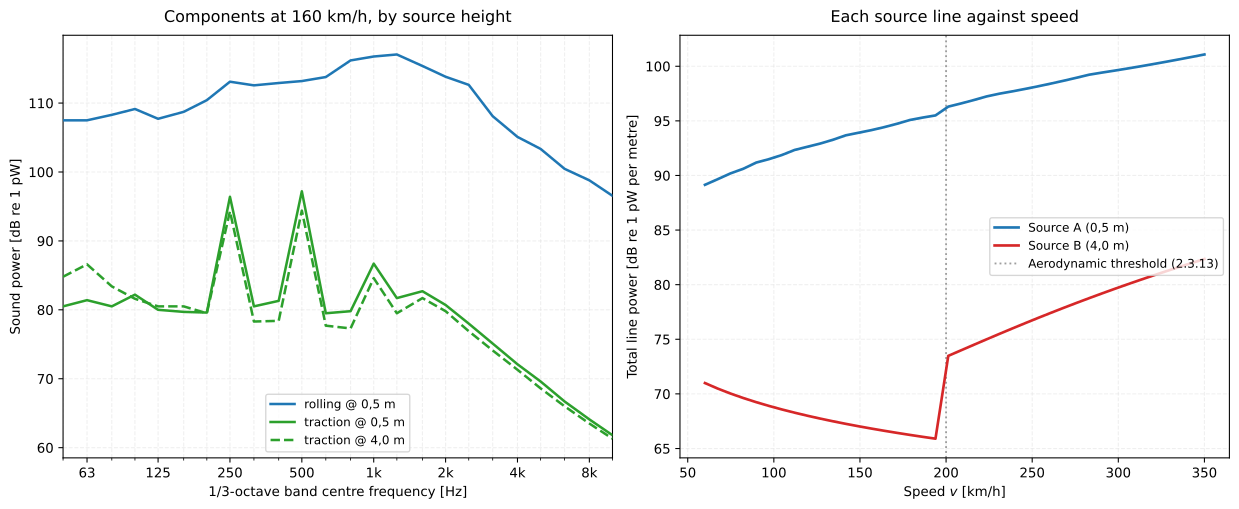

Left: the allocation table of this section, drawn. Rolling noise is the whole of source A at 160 km/h; traction is the only component present on both heights, and the aerodynamic and bridge entries of result.components come back as nan because neither is active here — which is the allocation rule showing itself. Right: source B is nearly flat and then steps, because aerodynamic noise is only modelled above 200 km/h; source A never stops rising. Source B does not overtake source A on this vehicle at any speed. The gap closes from 29.9 dB at 200 km/h to 18.7 dB at 350 km/h, and that closing is the sense in which the pantograph starts to matter.

Show the code for this figure

import matplotlib.pyplot as plt
import numpy as np

# `stock`, `track`, `railway_source_power` and `RailwayVehicle` come from the
# figure snippet above; the result carries its own frequency axes.
def total(bands):
    return 10.0 * np.log10(np.sum(10.0 ** (np.asarray(bands) / 10.0)))

fig, (left, right) = plt.subplots(1, 2, figsize=(12, 4.6))
result = railway_source_power(
    RailwayVehicle(stock, flow_rate=96.0, speed=160.0), track, phi=90.0, psi=10.0)
for name, spectrum in result.components.items():
    for row, height in ((0, "0,5 m"), (1, "4,0 m")):
        values = np.asarray(spectrum)[row]
        if np.any(np.isfinite(values)):
            left.semilogx(result.third_octave_frequencies, values,
                          label=f"{name} @ {height}")
left.set(xlabel="1/3-octave band [Hz]", ylabel="Sound power [dB]")
left.legend(fontsize="small")

speeds = np.linspace(60.0, 350.0, 30)
for row, label in [(0, "Source A (0,5 m)"), (1, "Source B (4,0 m)")]:
    right.plot(speeds, [
        total(railway_source_power(
            RailwayVehicle(stock, flow_rate=96.0, speed=float(v)),
            track, phi=90.0, psi=10.0).line_power[row]) for v in speeds],
        label=label)
right.axvline(200.0, ls=":", label="Aerodynamic threshold")
right.set(xlabel="Speed v [km/h]", ylabel="Total line power [dB/m]")
right.legend(fontsize="small")
plt.show()

3. Rolling noise: roughness in, sound power out

Rolling noise is the wheel and the rail exciting each other through the roughness of the two running surfaces. The method separates the cause from the radiation:

• cause: the rail roughness $L_{r,TR}$ (the second table of G-1, called G-1b here, selected by digit 2 of the track descriptor) and the wheel roughness $L_{r,VEH}$ (the first, G-1a, selected by the brake type, digit 3 of the vehicle descriptor), energy-summed and then filtered by the contact filter $A_3$ (Table G-2), which accounts for the finite size of the contact patch:

$$L_{R,\mathrm{TOT},i}=10{\log }_{10}\left(10^{L_{r,TR,i}/10}+10^{L_{r,VEH,i}/10}\right)+A_{3,i};$$

• radiation: three speed-independent transfer functions turn that roughness into sound power per axle, one for the track (Table G-3a, selected by the sleeper and rail-pad codes), one for the wheel (Table G-3b, selected by the wheel diameter) and one for the superstructure of a freight wagon (Table G-3c, which is 0,0 dB in every band):

$$L_{W,0,TR,i}=L_{R,\mathrm{TOT},i}+L_{H,TR,i}+10{\log }_{10}{N}_a,$$

and the same addition for the wheel and the superstructure. The three components are then energy-summed, and all three sit at source A.

The superstructure term applies to vehicle type a (freight) only. A minimum speed of 50 km/h, or 30 km/h for trams and light metro, is used to determine the roughness, which freezes the source spectrum below it; the flow term still uses the true speed. While a vehicle idles, rolling noise is excluded altogether.

4. The wavelength-to-frequency conversion

Roughness is tabulated against wavelength, and read at $\lambda =v/f$, so the whole roughness spectrum slides along the frequency axis as the train speeds up. That is the reason a fast train is bright and a slow one is not: the same millimetre-scale roughness excites a higher band.

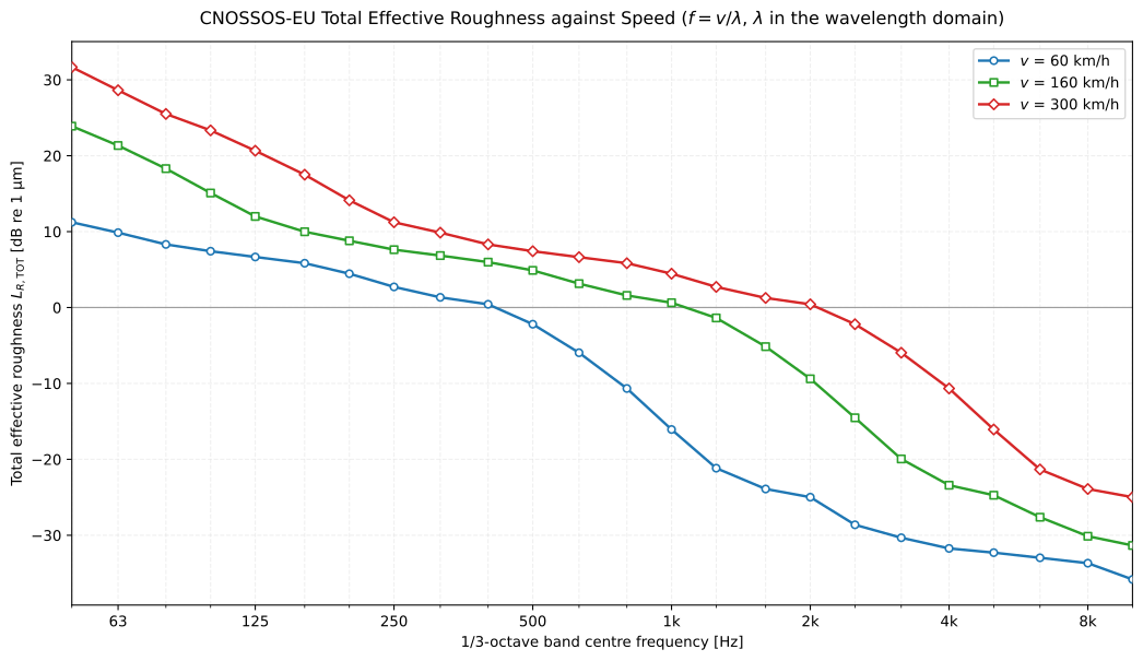
The same track and the same wheel at three speeds. The curve does not change shape, it slides: multiplying the speed by 2,7 moves it by rather more than an octave and lifts it, because the long wavelengths of an average network are the rough ones.

Show the code for this figure

import matplotlib.pyplot as plt
from phonometry import (
    RAILWAY_THIRD_OCTAVE_BANDS, BrakeType, ContactFilter, RailRoughnessClass,
    contact_filter, rail_roughness, roughness_to_frequency,
    total_effective_roughness, wheel_roughness,
)

rail = rail_roughness(RailRoughnessClass.NORMAL)
wheel = wheel_roughness(BrakeType.NON_TREAD)
filt = contact_filter(ContactFilter.LOAD_50_DIAMETER_920)

fig, ax = plt.subplots()
for speed in (60.0, 160.0, 300.0):
    total = total_effective_roughness(
        roughness_to_frequency(rail[1], rail[0], speed),
        roughness_to_frequency(wheel[1], wheel[0], speed),
        roughness_to_frequency(filt[1], filt[0], speed),
    )
    ax.semilogx(RAILWAY_THIRD_OCTAVE_BANDS, total, label=f"v = {speed:g} km/h")
ax.legend()
plt.show()

Two things about this conversion deserve to be stated plainly, because neither is settled by the Directive.

The speed is in metres per second. The published 2015 text says km/h in both places where the conversion appears, which would put the spectrum 3,6 times too low in frequency. The corrigendum of 2018 corrected both. This library implements the corrected form.

The interpolation rule is prose, not a formula. All the Directive says is that “the two corresponding 1/3 octave bands defined in the wavelength domain shall be averaged energetically and proportionally”, with no formula and no worked example. Two readings are shipped, and the default is the one that reproduces the Commission’s own reference source module:

from phonometry import RoughnessInterpolation

RoughnessInterpolation.PROPORTIONAL   # levels interpolated linearly in lambda
RoughnessInterpolation.ENERGY         # energies interpolated linearly in lambda

They differ by up to about 1 dB on a steep part of a spectrum. This is the single largest interpretation risk in the railway model, and any implementation that does not say which rule it uses is not comparable with another one.

A third, smaller ambiguity is handled without a switch. The 2021 amendment put the tables it replaced on the standard 1/3-octave wavelength series, but its point (20)(a) replaces “the second table” of G-1 only, so the wheel roughness of the first is still printed at 120, 12, 3,2 and 1,2 mm where every other table now reads 125, 12,5, 3,15 and 1,25 mm. Rather than forcing the two onto a common grid, each table is resampled on the grid the Directive prints for it.

5. Impact noise, and curve squeal

Impact noise from joints, switches and crossings is added as a fictitious extra roughness, energy-summed into the total before the transfer functions are applied (2.3.11). Table G-4 is given for one joint per 100 m, and any other density scales it (2.3.12):

$$L_{R,\mathrm{IMPACT},i}=L_{R,\mathrm{IMPACT}-\mathrm{SINGLE},i}+10{\log }_{10}\left(\frac{n_l}{0,01}\right).$$

For jointed track a default $n_l=0,01{\text{m}}^{-1}$ is prescribed. Impact noise is not modelled below the minimum speed, nor while idling. The increment applies from 50 m before the joint to 50 m after it, which is a segmentation instruction: the model gives the source strength, and it is up to the track segmentation to place it over the right 100 m.

Curve squeal is an excess added to the rolling-noise sound power at all frequencies. The rule is the one the 2021 amendment substituted, and it is not the 2015 one:

Vehicle	Condition	Excess
Train	$300\text{m}<R\le 500\text{m}$ over at least 50 m of curve	5 dB
Train	$R\le 300\text{m}$ over at least 50 m of curve	8 dB
Train	switch turnout with $R\le 300\text{m}$	8 dB
Tram	curve or switch turnout with $R\le 200\text{m}$	5 dB

from phonometry import curve_squeal_excess

curve_squeal_excess(280.0)                       # 8.0 dB
curve_squeal_excess(450.0)                       # 5.0 dB
curve_squeal_excess(280.0, tram=True)            # 0.0 dB, trams need R <= 200 m
curve_squeal_excess(280.0, track_length=20.0)    # 0.0 dB, the curve is too short

The 2015 text read “8 dB for R < 300 m and 5 dB for 300 m < R < 500 m”, which left the two endpoints with no rule at all even though the same paragraph scoped the effect to “curves with radius below or equal to 500 m”. The 2021 wording closes both intervals.

6. Traction and aerodynamic noise

Traction noise is tabulated per vehicle and per source height (Table G-5). The Directive models only two running conditions, constant speed (which it says is valid as well when the train accelerates or decelerates) and idling, and it takes the source strength at maximum load in both. Table G-5 therefore tabulates a single value per band and height, and the method reads it for both conditions: $L_{W,0,\mathrm{const},i}=L_{W,0,\mathrm{idling},i}$ is a consequence of how the table is printed, not a physical claim that an idling locomotive is as loud as a running one. Idling is only considered if trains idle for more than half an hour.

Aerodynamic noise is relevant only above 200 km/h and follows a logarithmic speed law about $v_0=300\text{km/h}$ (2.3.13, 2.3.14):

$$L_{W,0,i}=L_{W,0,h,i}(v_0)+{\alpha }_{h,i}{\log }_{10}\left(\frac{v}{v_0}\right),$$

with ${\alpha }_1={\alpha }_2=50$ in every band, so a doubling of speed adds 15,05 dB. Table G-6 is the reference spectrum of a 20 m vehicle at $v_0$: at the lower height it is broadband, at the upper one it is essentially silent except for a 1,6 kHz to 3,15 kHz plateau at 105 to 110 dB, which is the pantograph.

7. Source directivity

Each source is corrected in the two planes before the flow term is added (2.3.5). The horizontal correction is a dipole (2.3.15), 0 dB broadside and $10{\log }_{10}0,01=-20\text{dB}$ along the track:

$$\Delta L_{W,\mathrm{dir},\mathrm{hor},i}=10{\log }_{10}\left(0,01+0,99{\sin }^2\phi \right).$$

The vertical correction of source A (2.3.16) depends on the band, and it is one of the pieces the 2021 amendment rewrote. The current text drops the absolute-value bars of the 2015 form and makes the correction identically zero for $\psi \le 0$:

$$\Delta L_{W,\mathrm{dir},\mathrm{ver},i}=\frac{40}{3}\left[\frac{2}{3}\sin 2\psi -\sin \psi \right]{\log }_{10}\left(\frac{f_{c,i}+600}{200}\right),0<\psi <\pi /2,$$

and zero elsewhere. The two editions disagree over the whole lower half space, and also above about 41,4 degrees, where the bracket turns negative. Both are available, because comparing with a study computed before 2021 needs the old one:

from phonometry import DirectivityEdition, vertical_directivity

vertical_directivity(-30.0)                                        # zeros
vertical_directivity(-30.0, edition=DirectivityEdition.ORIGINAL_2015)  # positive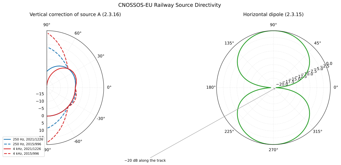

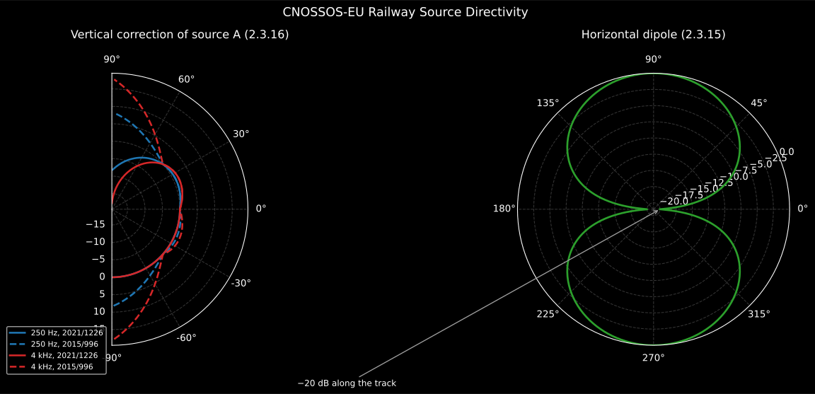
Left: the two editions agree only in the first quadrant below 41.4°, which is exactly where the bracket $\frac{2}{3}\sin 2\psi -\sin \psi$ is positive. Below the horizon the 2021 text returns 0 dB where the 2015 text returned up to +2.4 dB at 250 Hz and 60° below the horizon; above 41.4° the current form goes negative and the old one does not. A study computed before 2021 is not comparable band by band unless the edition is stated. Right: the horizontal dipole is worth 20 dB between a receiver beside the track and one at the end of it, which is why a track running towards a dwelling is a different problem from one running past it.

Show the code for this figure

import matplotlib.pyplot as plt
import numpy as np

# `vertical_directivity` and `DirectivityEdition` come from the snippet above;
# the horizontal dipole is formula (2.3.15) itself, one line of numpy.
psi = np.linspace(-89.0, 89.0, 179)
bands = {7: "250 Hz", 19: "4 kHz"}       # indices into the 24 third-octaves
fig, (left, right) = plt.subplots(1, 2, subplot_kw={"projection": "polar"},
                                  figsize=(12, 5.0))
for band, name in bands.items():
    for edition, style in [(DirectivityEdition.CURRENT, "-"),
                           (DirectivityEdition.ORIGINAL_2015, "--")]:
        values = [float(vertical_directivity(float(a), edition=edition)[band])
                  for a in psi]
        left.plot(np.radians(psi), values, style,
                  label=f"{name}, {edition.value}")
left.legend(fontsize="small", loc="lower left")

phi = np.radians(np.linspace(0.0, 360.0, 361))
right.plot(phi, 10.0 * np.log10(0.01 + 0.99 * np.sin(phi) ** 2))
right.set_title("Horizontal dipole (2.3.15)", fontsize="small")
plt.show()

At source B, only the aerodynamic source is directional, $10{\log }_{10}({\cos }^2\psi )$ for $\psi <0$ (2.3.17); everything else at 4,0 m is omni-directional, and so is bridge noise at 0,5 m.

One point of interpretation: 2.3.15 offers the dipole “by default … for rolling, impact, squeal, braking, fans and aerodynamic effects”. Traction noise other than the fans is not in that list, and the Directive gives no other horizontal directivity for it. This library applies the dipole to every source, which is what the Commission’s reference source module does.

8. Bridges

On a bridge the deck radiates too. The 2015 text added a constant to the rolling noise, 1 dB for concrete or masonry and 4 dB for steel with ballasted track. The 2021 amendment replaced that with a separate source, built exactly like a rolling-noise component but with the bridge transfer function of Table G-7 (2.3.18):

$$L_{W,0,\mathrm{bridge},i}=L_{R,\mathrm{TOT},i}+L_{H,\mathrm{bridge},i}+10{\log }_{10}{N}_a.$$

The rolling noise of the vehicle on the bridge is still computed normally, with the transfer function of the track system that is actually on the bridge; the bridge term is added to it. It sits at source A and is omni-directional, which the amendment states explicitly.

Table G-7 has exactly two columns, and the Directive labels them by the A-weighted bridge excess they stand for rather than by a construction type: BridgeType.PLUS_10_DBA selects the “+10 dB(A)” column and BridgeType.PLUS_15_DBA the “+15 dB(A)” one. There is no third column and no interpolation, so choosing between them is a judgement about the deck, made before the calculation and recorded with it.

from phonometry import BridgeType, RailwayTrack, bridge_transfer

RailwayTrack(
    rail_roughness=..., track_transfer=...,
    bridge_transfer=bridge_transfer(BridgeType.PLUS_10_DBA),   # Table G-7, col. 1
)

9. Handing the source to a propagation model

The railway source is derived in 1/3 octave bands and then energy-summed into octave bands for propagation, which is what 2.3.2 requires and what (EU) 2021/1226 point (1) made explicit. The result object carries both:

The result here is the one the section 2 snippet built (open its <details> block for the vehicle and track it describes). Row 0 is source A at 0,5 m and row 1 source B at 4,0 m, the h = 1 and h = 2 of the section 2 table:

result.third_octave_line_power   # (2, 24), the two heights in 1/3 octaves
result.line_power                # (2, 8), the same in octave bands
result.total_line_power          # (8,), the two heights energy-summed
result.components["rolling"]     # the per-source breakdown, before directivity
result.frequencies               # the 8 octave centres
result.third_octave_frequencies  # the 24 third-octave centres

A component that is not active at the modelled condition comes back as nan rather than as a floor value, so components["aerodynamic"] below 200 km/h and components["bridge"] off a bridge are both all-nan.

Splitting a source line into equivalent point sources is, in the words of section 2.5.3, “outside the scope of the current methodology”: a point source standing for a segment of length $dL$ simply carries $L_{W,\mathrm{eq},\mathrm{line},i}^{\prime }+10{\log }_{10}(dL)$, which is arithmetic.

CNOSSOS-EU has its own propagation method in section 2.5 of Annex II, and it is not ISO 9613-2. Chaining a CNOSSOS emission onto the ISO 9613-2 propagation of this library is a legitimate engineering estimate, but it is not the normative CNOSSOS chain and must not be reported as one.

10. What is pinned against digits, and what is not

Annex II prints no worked example and no check value anywhere in 2.3 or Appendix G, so it is worth being explicit about what the agreement in the test suite measures.

Verified against published digits. Every Appendix G table, against the Official Journal text of the instrument that enacted it. And the whole chain of equations end to end, against the emission test workbook the European Commission published with its reference source module: feeding the shipped equations the 2015 coefficient database that workbook was computed with reproduces all 34 560 published rows of the twenty vehicles whose catalogue entries are well formed, that is 17 280 cases at both source heights, to 0,0055 dB, inside the two decimals it prints. A hundred and twenty-three of those cases are committed to the repository and run in CI. The three vehicles left out are described in tests/data/cnossos/README.md: their rows record defects of the reference program, not of the method.

That agreement resolves the loud parts of the database and not the quiet ones: a coefficient twenty decibels below its neighbour does not move the total, so the placeholder rows of the reference catalogue and the source-A traction column, which rolling noise always covers, are carried by the test set without being constrained by it. tests/data/cnossos/README.md reports the measurement.

Verified as equations times transcribed tables, not end to end. Everything the 2021 amendment changed. The workbook predates it, so the new curve-squeal rule, the bridge transfer function, the current vertical directivity and the five replaced tables are each pinned individually, by transcription and by closed-form assertion, but their combination has never been checked against an independent published result.

Not anchored on any oracle. The choice of interpolation rule in section 4; the proportional distribution of traction sound power when a real component sits between the two model heights, for which the Directive gives no formula; and the segmentation of a line into point sources, which the method declares out of scope.

What this guide covers

• Covered

  Section 2.3 of Annex II to Directive 2002/49/EC in the consolidated text: the vehicle and track descriptors of Tables [2.3.a] and [2.3.b], the traffic-flow line power (2.3.1, 2.3.2, 2.3.4), the directional sound power (2.3.5), rolling noise (2.3.6 to 2.3.10), impact noise (2.3.11, 2.3.12), curve squeal, traction noise, aerodynamic noise (2.3.13, 2.3.14), the source directivity (2.3.15 to 2.3.17) and bridge noise (2.3.18), together with the whole Appendix G database, through railway_source_power and the component functions around it.

• Not covered

  The road source (2.2 and Appendix F), the industrial source (2.4 and Appendix H), the aircraft source (2.6 and 2.7) and the CNOSSOS-EU propagation method of section 2.5, which is a different model from the ISO 9613-2 one implemented in this library. Rail roughness classes N (not well maintained) and B (bad condition) carry no spectrum in Appendix G and have to be supplied by the Member State. The other railway sources of 2.3.3, such as depots, stations and loudspeakers, are treated by the industrial method.

See also

• API reference: environment.sources.cnossos_rail.
• Outdoor Sound Propagation: the ISO 9613-2 chain that carries a source power to a receiver.
• Environmental noise levels: the $L_{den}$ and $L_{night}$ indicators the resulting maps are drawn for.

References

• European Union. (2015). Commission Directive (EU) 2015/996 establishing common noise assessment methods according to Directive 2002/49/EC of the European Parliament and of the Council (Directive (EU) 2015/996). Replaces Annex II of Directive 2002/49/EC with the CNOSSOS-EU methods. The implemented railway source is section 2.3 (formulae 2.3.1 to 2.3.18) with the coefficient database of Appendix G.
• European Union. (2018). Corrigendum to Commission Directive (EU) 2015/996 (OJ L 5, 10.1.2018, p. 35). Replaces the whole of Appendix G and corrects the railway roughness conversion, where the published text read km/h for a speed that has to be in metres per second.
• European Union. (2021). Commission Delegated Directive (EU) 2021/1226 amending, for the purposes of adapting to scientific and technical progress, Annex II to Directive 2002/49/EC as regards common assessment methods for noise (Directive (EU) 2021/1226). The amendment in force since 31 December 2021. Replaces Tables G-1b, G-2, G-3a, G-4 and G-7, substitutes a new curve-squeal rule and a new bridge model, and rewrites the vertical directivity of source A.
• International Organization for Standardization. (1996). Acoustics — Attenuation of sound during propagation outdoors — Part 2: General method of calculation (ISO 9613-2:1996). The propagation model used here to carry the emission to a receiver. CNOSSOS-EU has its own propagation method in section 2.5 of Annex II, which is not ISO 9613-2.
• Kephalopoulos, S., Paviotti, M., & Anfosso-Lédée, F. (2012). Common noise assessment methods in Europe (CNOSSOS-EU) (EUR 25379 EN). Publications Office of the European Union. https://doi.org/10.2788/31776The Joint Research Centre reference report the Directive text descends from, with the IMAGINE measurement campaigns behind the Appendix G coefficients.