Spherical ground effect and advanced barriers
Standards: EN 1793Key references: Attenborough & Van Renterghem 2021Salomons 2001Bies et al. 2017Kurze & Anderson 1971Hadden & Pierce 1981
The ISO 9613-2 general method folds
the ground and barrier terms into tabulated, energy-based corrections. This page
covers the underlying wave acoustics in
phonometry.environment.propagation.ground_barriers: the spherical-wave reflection
coefficient of a finite-impedance ground (Weyl-Van der Pol) and the
wave-theoretic diffraction of a screen, both in a homogeneous
(non-refracting, non-turbulent) atmosphere. These are the physical core of the
Nord2000 / CNOSSOS ground and barrier models, and they resolve the
frequency-dependent interference structure the octave-band /
terms smooth away.
1. Spherical-wave ground effect (Weyl-Van der Pol)
Section titled “1. Spherical-wave ground effect (Weyl-Van der Pol)”The sound field of a point source above a locally reacting ground is the sum of a direct wave and a reflected wave weighted by the spherical-wave reflection coefficient (Attenborough Eq. 2.40a; Salomons Eq. 3.2):
with the source-receiver distance and the image-source distance. The coefficient (Attenborough Eq. 2.40c; Salomons Eq. D.58) corrects the plane-wave coefficient for the curvature of the wavefront:
Here is the ground surface impedance normalized by , is
the angle of incidence from the ground normal
(), and the boundary-loss factor is
written through the scaled complementary error function
, i.e. the Faddeeva function
scipy.special.wofz. The second term of is the ground wave that keeps
the field finite at grazing incidence, where and a plane-wave
model would predict silence
(Salomons Eqs. D.57, D.59, D.60).
The relative sound level (the excess attenuation, dB re free field) is (Salomons Eq. 3.4):
import numpy as npfrom phonometry import environment
bands = np.array([63., 125., 250., 500., 1000., 2000., 4000., 8000.])
# Grassland (effective flow resistivity sigma = 200 kPa.s/m^2), source 1 m and# receiver 1.5 m high, 50 m apart. The impedance comes from the Delany-Bazley# porous model of phonometry.materials (a semi-infinite ground).# Argument order: frequencies, source_height, receiver_height, distance.res = environment.ground_effect(bands, 1.0, 1.5, 50.0, flow_resistivity=2e5)print(res.excess_attenuation)     # the ground dip (dB re free field)print(res.reflection_coefficient) # complex Q per bandres.plot()                        # excess attenuation vs frequency
The ground impedance is either derived from an effective flow_resistivity
(via the delany_bazley or miki model of
phonometry.materials, which model a
semi-infinite porous ground) or supplied directly as a normalized complex
impedance (a scalar, per-band array, or a PorousMediumResult). A plain
impedance value is taken in the convention of Salomons, in
which a passive ground has ; the porous models of
phonometry.materials work in the opposite convention
(), so anything obtained
from them (a flow_resistivity or a PorousMediumResult) is conjugated
internally before it enters the Weyl-Van der Pol formulas.
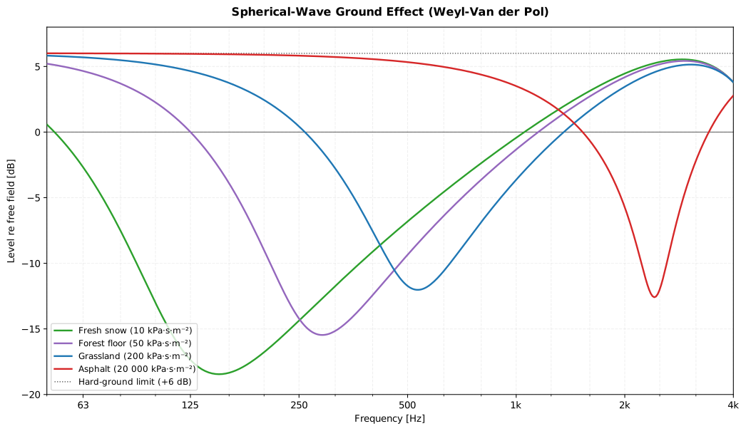
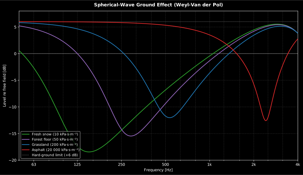
Softer ground means a deeper dip at a lower frequency: the dip tracks the effective flow resistivity across more than a decade, and only asphalt stays near the +6 dB hard-ground limit across the speech range. Note the unit: the flow resistivity is a resistivity in Pa·s/m², not a pressure.
Show the code for this figure
import matplotlib.pyplot as pltimport numpy as npfrom phonometry import environment
freqs = np.geomspace(50.0, 4000.0, 400)grounds = [    ("Fresh snow (10 kPa·s·m⁻²)", 10e3, "#2ca02c"),    ("Forest floor (50 kPa·s·m⁻²)", 50e3, "#9467bd"),    ("Grassland (200 kPa·s·m⁻²)", 200e3, "#1f77b4"),    ("Asphalt (20 000 kPa·s·m⁻²)", 20000e3, "#d62728"),]fig, ax = plt.subplots(figsize=(11, 6.4))for label, sigma, color in grounds:    res = environment.ground_effect(freqs, 1.0, 1.5, 50.0, flow_resistivity=sigma)    ax.plot(freqs, res.excess_attenuation, color=color, label=label)ax.axhline(6.0, color="k", ls=":", label="Hard-ground limit (+6 dB)")ax.axhline(0.0, color="k", lw=0.8)ax.set_xscale("log")ax.set_xlabel("Frequency [Hz]")ax.set_ylabel("Level re free field [dB]")ax.legend()plt.show()
Limits reproduced by the implementation (each a pinned test or conformance anchor): an acoustically hard ground () gives , , and , so reaches +6 dB in phase; the effective flow resistivity tends to that hard ground; grazing incidence () gives ; and the ground effect is reciprocal under an exchange of source and receiver heights.
The ground wave is easiest to see by taking the geometry towards grazing and watching and come apart.
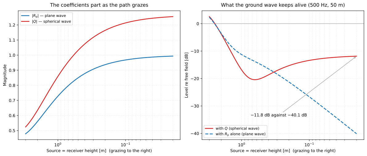
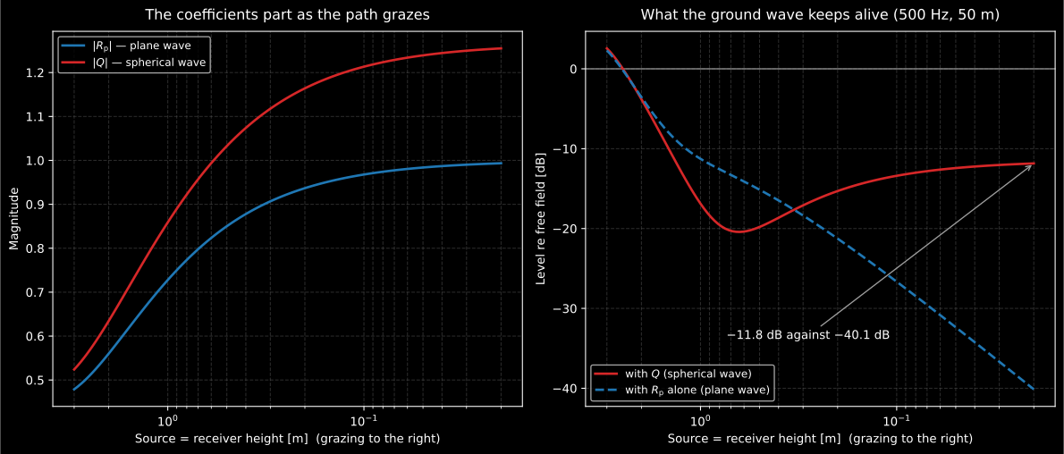
At 3 m of height the two coefficients agree to within a few per cent and the ground wave is irrelevant. By 0.02 m, has reached (magnitude 0.993 at 179.6°) and a plane-wave model predicts dB, near silence. The spherical coefficient reaches instead and the field settles at dB. That 28 dB is what the Faddeeva term buys, and it is why a grazing outdoor path is audible at all.
Show the code for this figure
import matplotlib.pyplot as pltimport numpy as np
# `ground_effect` is imported by the snippet above.heights = np.geomspace(3.0, 0.02, 60)c0, f, d = 343.0, 500.0, 50.0k = 2 * np.pi * f / c0q_mag, rp_mag, dl_q, dl_p = [], [], [], []for h in heights:    res = environment.ground_effect([f], h, h, d, flow_resistivity=2e5, model="miki")    rp = res.plane_reflection_coefficient[0]    q = res.reflection_coefficient[0]    phase = np.exp(1j * k * (float(res.r_reflected) - float(res.r_direct)))    ratio = float(res.r_direct) / float(res.r_reflected)    rp_mag.append(abs(rp))    q_mag.append(abs(q))    dl_q.append(20 * np.log10(abs(1 + q * ratio * phase)))    dl_p.append(20 * np.log10(abs(1 + rp * ratio * phase)))
fig, (left, right) = plt.subplots(1, 2, figsize=(11, 4.6))left.semilogx(heights, rp_mag, label="|Rp| (plane wave)")left.semilogx(heights, q_mag, label="|Q| (spherical wave)")left.invert_xaxis()left.set(xlabel="Source = receiver height [m]", ylabel="Magnitude")left.legend()right.semilogx(heights, dl_q, label="with Q")right.semilogx(heights, dl_p, label="with Rp only")right.invert_xaxis()right.set(xlabel="Source = receiver height [m]",          ylabel="Level re free field [dB]")right.legend()plt.show()
Choosing the ground impedance
Section titled “Choosing the ground impedance”Both one-parameter models are being evaluated far below their published fit
range for any outdoor ground, and the PorousAbsorberWarning these calls raise
says so: the range is with , and the
grassland above sits at at 63 Hz and 0.024 at 4 kHz;
the asphalt curve of the figure never enters the range at all. Below the range the
Delany-Bazley regression is an extrapolation whose classic failure is a negative
real part of the surface impedance; Miki is the passivity-constrained refit
to prefer there (see the fit-range paragraph of
Porous absorbers). The
choice is not cosmetic: on the case above, model="miki" moves the excess
attenuation by up to 3.6 dB (250 Hz band: 0.43 dB with Delany-Bazley,
−3.18 dB with Miki).
Typical effective flow resistivities, the ranges the figure above illustrates: fresh snow ≈ 10, forest floor ≈ 50, grassland and pasture ≈ 150-300, compacted soil and gravel ≈ 1000-3000, asphalt and concrete > 20 000 kPa·s/m².
For a real site, fit to a short-range level-difference measurement between two microphone heights over the surface (the template method of ANSI/ASA S1.18). The fitted value is an effective, model-bound parameter: it must be quoted with the impedance model it was fitted with, and it is not the EN 29053 airflow resistivity of the same material.
2. Advanced barrier diffraction
Section titled “2. Advanced barrier diffraction”Three levels of screening beyond the ISO 9613-2 term are provided by
barrier_insertion_loss and its building blocks.
Kurze-Anderson closed form. The insertion loss of a thin screen as a function of the Fresnel number (Bies Eq. 5.134, with and the two segments of the shortest source-edge-receiver path and the straight distance) is (Bies Eq. 5.138; Kurze & Anderson 1971):
which tends to 5 dB at the shadow boundary and approximates Maekawa’s point-source curve within about 1.5 dB.
The clip below is that formula as a field. It is the 2D FDTD solver run twice on one 12 × 7 m half-space over rigid ground with a thin rigid screen 2.5 m tall, once at 100 Hz and once at 500 Hz, each with a barrier-free reference run over the same ground so the annotated insertion loss is a true one. The geometry fixes the path difference at 1.06 m for the receiver it marks, so the Fresnel number is at 100 Hz and at 500 Hz (the same screen, a factor of five apart in purely because changed), and the field shows what that buys: about 8 dB against about 17 dB. Two things are worth watching for. The edge of the lit region running down from the top of the screen is the shadow boundary, the locus where the formula bottoms out at 5 dB; and inside the shadow the field is a cylindrical wave centred on the top of the screen, which is what “the edge acts as a secondary source” looks like. One caveat: the ground in the clip is perfectly rigid, so it shows diffraction alone and none of the finite-impedance ground effect of section 1; the coherent four-path model below adds that, and its curve swings tens of decibels where this one is smooth.
A 2D FDTD simulation of a point source behind a thin 2.5 metre rigid barrier on reflecting ground, at 100 Hz and 500 Hz side by side. The long wavelength diffracts over the edge and fills the shadow zone with an insertion loss near 8 dB, while the short wavelength is cast into a deep clean shadow of about 17 dB.
A 2D FDTD simulation of a point source behind a thin 2.5 metre rigid barrier on reflecting ground, at 100 Hz and 500 Hz side by side. The long wavelength diffracts over the edge and fills the shadow zone with an insertion loss near 8 dB, while the short wavelength is cast into a deep clean shadow of about 17 dB.
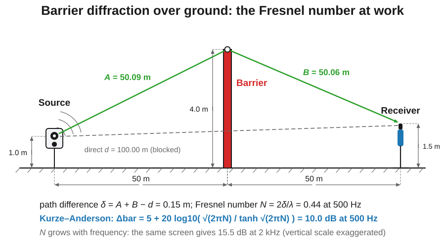
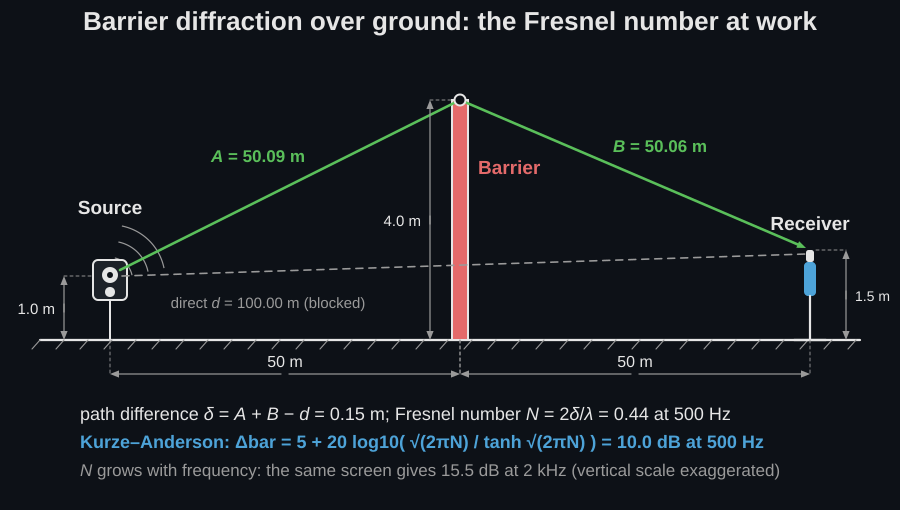
The thin-screen methods share the same three geometric quantities: the two diffracted segments over the edge and the straight path they replace. Drawn on the 4 m screen of the snippets, they differ by just 0.15 m.
from phonometry import environment
environment.kurze_anderson_attenuation(0.0)     # 5.0 dB at the shadow boundary
# A 4 m barrier 50 m from a 1 m source, receiver 1.5 m high at 100 m.il = environment.barrier_insertion_loss(bands, 1.0, 50.0, 4.0, 100.0, 1.5,                                        method="kurze_anderson")il.plot()                           # insertion loss vs frequency
Exact rigid half-plane. With method="exact" the wave-theoretic insertion
loss of a rigid thin screen is used: the compact Fresnel-integral form of the
MacDonald / Hadden & Pierce solution (Attenborough Eqs. 9.19-9.20), built from
the auxiliary Fresnel functions. It gives 6 dB at the shadow boundary (the
field is exactly halved, the flat-wedge limit) and tracks Kurze-Anderson through
the shadow zone.
Thick barriers. A thickness (top width ) moves the second diffraction
edge downstream and lengthens the diffracted path to , the double-edge
Fresnel number of Bies Eq. 5.157. The
improvement is monotone but it is small, and the reason is geometric: is now
measured from the far edge, so most of what the top width adds it also gives
back. On the 4 m screen of this page, a 4 m top width is worth 0.08 dB at
500 Hz and 0.14 dB at 8 kHz; even 30 m of width only reaches 1.2 dB.
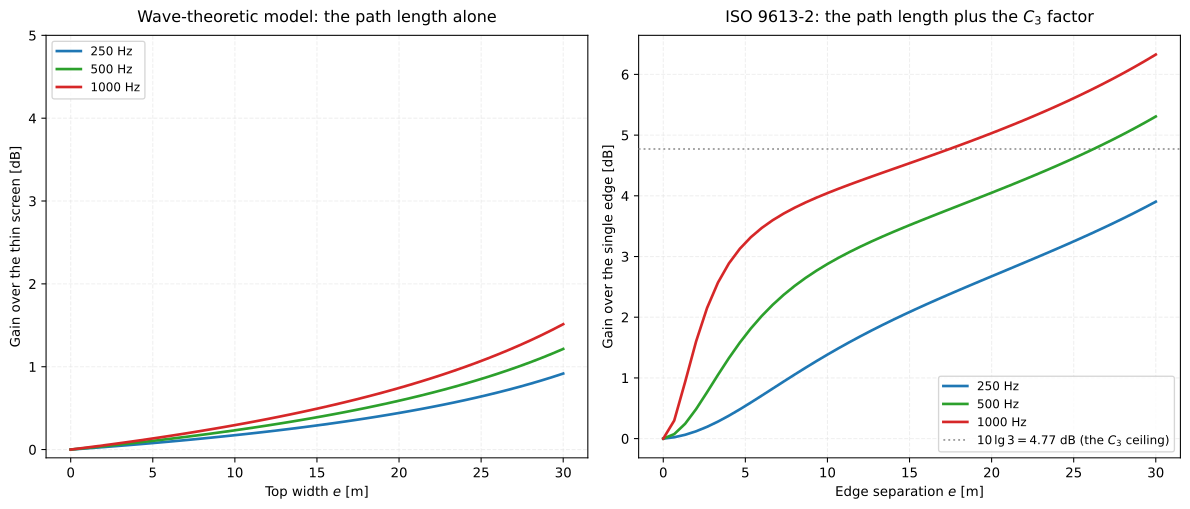
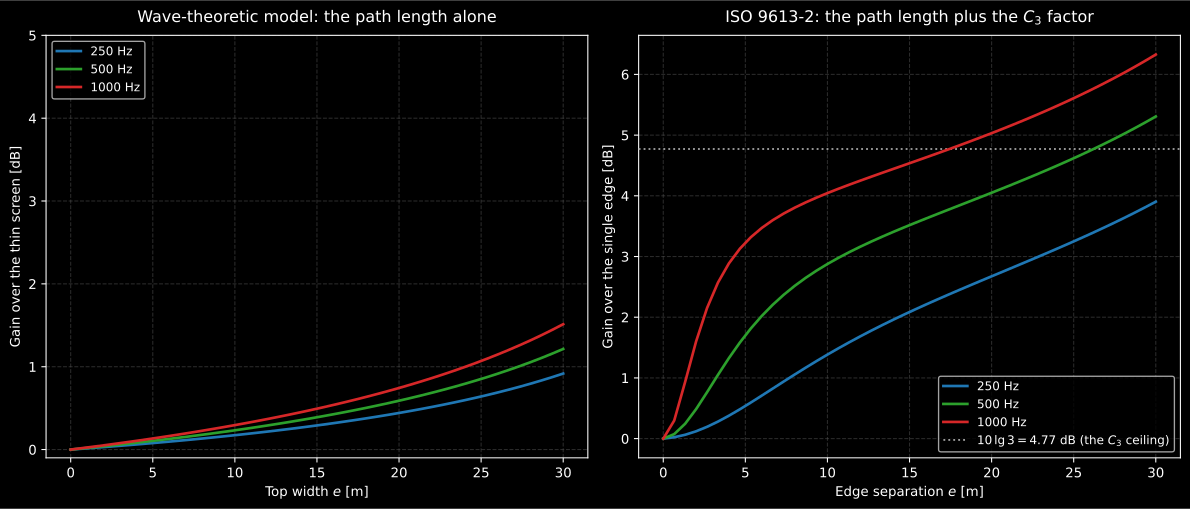
The path-length effect alone is worth a fraction of a decibel at road-traffic distances. ISO 9613-2 credits a well-separated double edge with a separate factor that rises from 1 towards 3, worth up to dB, which the wave-theoretic model here does not include: for the same 4 m top width goes from 7.6 dB to 9.0 dB at 500 Hz. Neither number licenses building a berm and expecting the ISO bonus from this page’s model.
Show the code for this figure
import matplotlib.pyplot as pltimport numpy as np
# `barrier_insertion_loss` is imported by the snippet above.widths = np.linspace(0.0, 30.0, 40)fig, ax = plt.subplots()for freq in (250.0, 500.0, 1000.0):    thin = float(environment.barrier_insertion_loss(        [freq], 1.0, 50.0, 4.0, 100.0, 1.5, method="exact").insertion_loss[0])    gain = [0.0 if e == 0.0 else float(environment.barrier_insertion_loss(        [freq], 1.0, 50.0, 4.0, 100.0, 1.5, method="exact",        thickness=e).insertion_loss[0]) - thin for e in widths]    ax.plot(widths, gain, label=f"{freq:g} Hz")ax.set_xlabel("Top width e [m]")ax.set_ylabel("Gain over the thin screen [dB]")ax.legend()plt.show()
Coherent barrier on the ground. With a ground_impedance (or a
ground_flow_resistivity) the four source-image / receiver-image diffracted
paths are combined coherently, each ground reflection weighted by the
spherical-wave coefficient above (Attenborough Ch. 9; Bies Sec. 5.3.5).
This exposes the ground-barrier interference structure that a purely energetic
sum of and cannot. As a first-order simplification a single
(over the
overall source-receiver geometry) weights every bounce rather than a separate
coefficient per image path; the model is coherent and reciprocal but not a full
boundary-element solution.
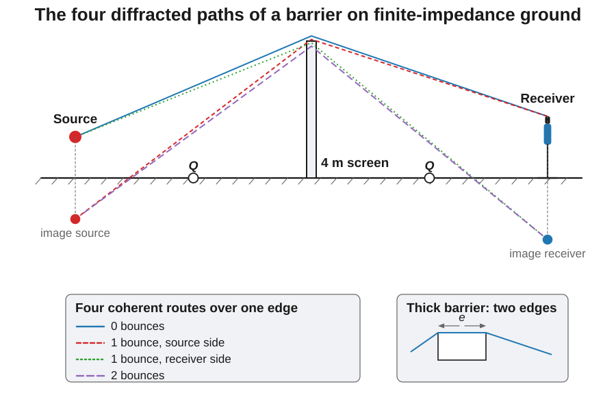
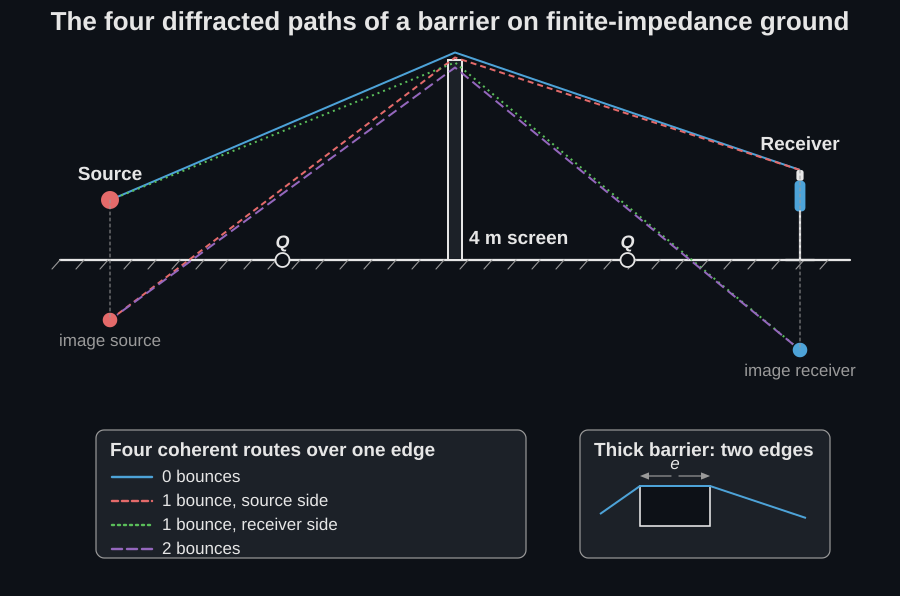
il = environment.barrier_insertion_loss(bands, 1.0, 50.0, 4.0, 100.0, 1.5, method="exact", ground_flow_resistivity=2e5)il.ground # True: the four-path coherent ground model was appliedil.plot()The three models side by side on the same geometry tell the whole story: the Kurze-Anderson fit and the exact half-plane track each other to within about 1.5 dB across two decades of Fresnel number, while the coherent ground model swings tens of decibels around them, up where the barrier removes the ground-effect dip of the unscreened path, down where the four diffracted paths interfere destructively.
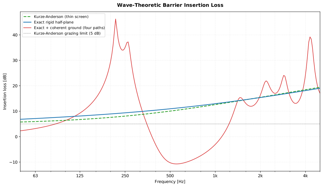
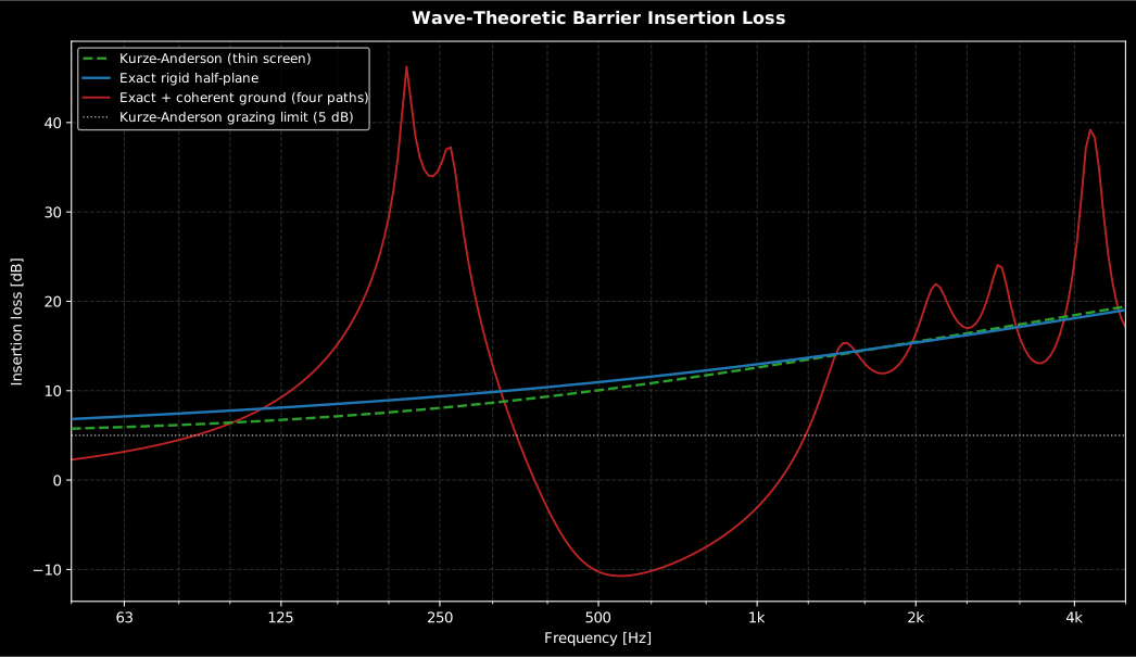
The two thin-screen models never separate by more than about 1.5 dB, so the choice between them barely matters. The coherent ground curve is a different kind of object: it swings from above +45 dB near 230 Hz, where the barrier removes the unscreened path’s own ground dip, to below −10 dB near 550 Hz, where the four diffracted paths cancel. Both extremes are narrowband and neither is a design value.
Show the code for this figure
import matplotlib.pyplot as pltimport numpy as npfrom phonometry import environment
# The 4 m barrier of the snippets above, on a fine frequency grid.freqs = np.geomspace(50.0, 5000.0, 240)il_ka = environment.barrier_insertion_loss(freqs, 1.0, 50.0, 4.0, 100.0, 1.5,                                           method="kurze_anderson")il_ex = environment.barrier_insertion_loss(freqs, 1.0, 50.0, 4.0, 100.0, 1.5,                                           method="exact")il_gr = environment.barrier_insertion_loss(freqs, 1.0, 50.0, 4.0, 100.0, 1.5,                                           method="exact", ground_flow_resistivity=2e5)fig, ax = plt.subplots(figsize=(11, 6.4))ax.semilogx(freqs, il_ka.insertion_loss, "--", label="Kurze-Anderson (thin screen)")ax.semilogx(freqs, il_ex.insertion_loss, label="Exact rigid half-plane")ax.semilogx(freqs, il_gr.insertion_loss, label="Exact + coherent ground (four paths)")ax.axhline(5.0, color="k", ls=":", label="Kurze-Anderson grazing limit (5 dB)")ax.set(xlabel="Frequency [Hz]", ylabel="Insertion loss [dB]")ax.legend()plt.show()
All three curves share the same base geometry, and .plot_geometry() draws
it to scale: at these road-traffic distances the 4 m screen is a sliver. For
the thin-screen curves the 0.15 m path difference combines with wavelength in
the Fresnel number; the coherent-ground curve also depends on ground
impedance and image-path interference.
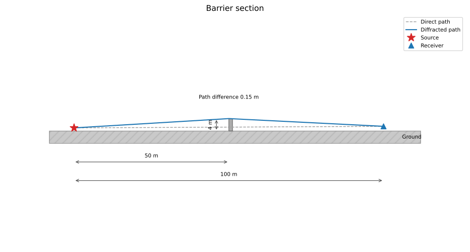
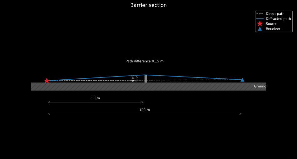
Drawn to scale the screen almost vanishes: the diffracted path over the top is only 0.15 m longer than the blocked direct path, and that difference is the geometric input of the Fresnel number that the thin-screen methods above key on.
Show the code for this figure
import matplotlib.pyplot as pltimport numpy as npfrom phonometry import environment
freqs = np.geomspace(50.0, 5000.0, 240)il = environment.barrier_insertion_loss(freqs, 1.0, 50.0, 4.0, 100.0, 1.5)
# One line: the section to scale, with the path-length difference annotated.il.plot_geometry()plt.show()
ground_effect() and barrier_insertion_loss() parameters
Section titled “ground_effect() and barrier_insertion_loss() parameters”Both entry points take their distances along the ground from the source, and
neither takes a distance from the barrier. That is the trap worth naming: in
barrier_insertion_loss(bands, 1.0, 50.0, 4.0, 100.0, 1.5) the receiver is
100 m from the source, i.e. 50 m past the screen, not 100 m past it. The two
functions also spell the same option differently (model= on ground_effect,
ground_model= on barrier_insertion_loss) and order their geometry
differently, which is why the two positional calls on this page are not
parallel.
ground_effect parameter | Type / shape | Units | Range / default | Notes |
|---|---|---|---|---|
frequencies | scalar or 1D array | Hz | > 0 | Narrowband: no band smoothing |
source_height | float | m | ≥ 0 | |
receiver_height | float | m | ≥ 0 | (before the distance) |
distance | float | m | > 0 | Horizontal source-receiver distance |
impedance | array, PorousMediumResult or None | — | None | Normalized in the convention |
flow_resistivity | float or None | Pa·s/m² | None | Effective ; feeds the porous model |
model | "delany_bazley" | "miki" | — | "delany_bazley" | Prefer "miki" below the fit range |
speed_of_sound / air_density | float | m/s, kg/m³ | 343.0 / 1.205 |
barrier_insertion_loss parameter | Type / shape | Units | Range / default | Notes |
|---|---|---|---|---|
frequencies | scalar or 1D array | Hz | > 0 | |
source_height | float | m | ≥ 0 | |
barrier_distance | float | m | > 0 | Source to the (near) edge, along the ground |
barrier_height | float | m | > 0 | Edge height above the ground |
receiver_distance | float | m | > barrier_distance (+ thickness) | Measured from the source |
receiver_height | float | m | ≥ 0 | (after the distance) |
method | "kurze_anderson" | "exact" | — | "exact" | "exact" is the rigid half-plane |
thickness | float or None | m | None | Top width ; double edge |
ground_impedance | array, PorousMediumResult or None | — | None | Selects the coherent four-path model |
ground_flow_resistivity | float or None | Pa·s/m² | None | Same, from an effective |
ground_model | "delany_bazley" | "miki" | — | "delany_bazley" | Note the name: not model= |
speed_of_sound / air_density | float | m/s, kg/m³ | 343.0 / 1.205 |
A ground argument requires method="exact"; method="kurze_anderson" with a
ground raises ValueError.
Choosing a model, and what none of them models
Section titled “Choosing a model, and what none of them models”Which one to use. Kurze-Anderson for an octave-band engineering estimate, where its ±1.5 dB against the exact solution is far inside the uncertainty of everything else in the chain. The exact rigid half-plane when the behaviour near the shadow boundary matters (it gives 6 dB there against Kurze-Anderson’s 5 dB, and the 6 dB is the physically correct halved field). The coherent four-path model only when the narrowband interference structure is the question: never raw as a design value.
The coherent curve must be averaged before it means anything. It is a coherent, narrowband, fully deterministic result. Real atmospheric turbulence decorrelates the four paths, a real source has bandwidth, and a real receiver moves; all three wash out the extremes. A +45 dB narrowband insertion loss is not a barrier that removes 45 dB, it is a frequency at which the unscreened path happened to sit in its own ground dip. Band-average the curve, or read it as structure rather than as a level.
All four models are two-dimensional endless screens. A real barrier of finite length lets sound flank around its ends, and two parallel barriers either side of a road reflect between each other and lose several decibels of their nominal performance. Neither effect exists in any model on this page.
Diffraction is the screening limit, not the realised one. The insertion loss a built barrier delivers is the smaller of the diffraction result and the transmission loss of the panel itself, and the obstacle has to qualify as a barrier in the first place: surface density, a closed surface, and a horizontal extent normal to the path larger than the wavelength. Those qualifying rules are stated in the “Barrier pitfalls” section of Outdoor Sound Propagation; they apply here unchanged.
3. What the product declaration says (EN 1793)
Section titled “3. What the product declaration says (EN 1793)”Everything above is the barrier as physics. A barrier on sale is a product, and what its declaration carries is two integers, neither of them a diffraction: how much of the sound reaching it comes back across the road, and how much of it goes through. Both are weighted by a spectrum nobody measures on site, the normalised traffic noise spectrum of EN 1793-3: eighteen one-third octave bands from 100 Hz to 5 kHz, peaking at 1 kHz and twelve decibels down at either end.
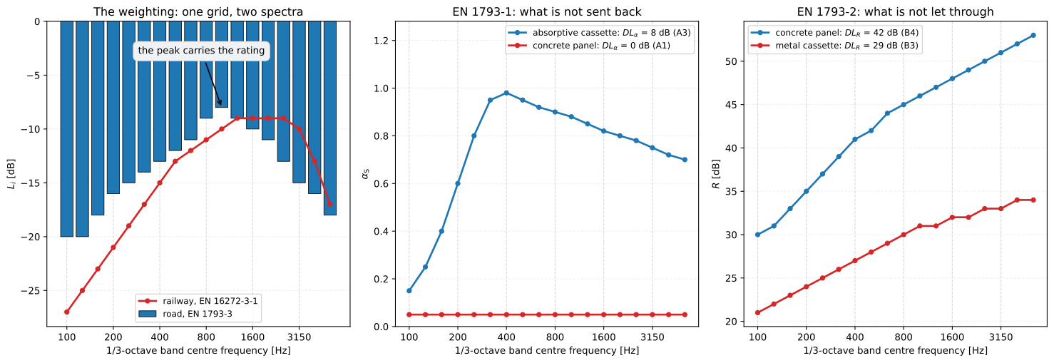
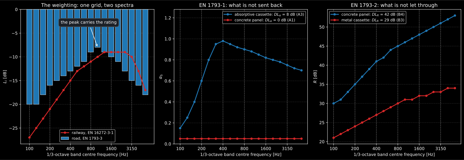
The weighting on the left decides everything, and there are two of them: a road device is judged by what it does around 1 kHz, a railway one by what it does between 1,25 and 2,5 kHz.
EN 1793-1 rates absorption as the energy the device does not send back:
A reverberation-room can pass one band by band, which would
push the weighted ratio past 1 and leave the logarithm without an argument.
Clause 5 says so and fixes it: the ratio is limited to 0,99, so no device can
rate above 20 dB however absorptive it measures. sound_absorption_rating
warns when that limit is what answered instead of the measurement.
EN 1793-2 rates airborne insulation with the same weighting, on the transmitted energy instead:
from phonometry import environment
# A cassette with mineral wool behind a perforated face, in the eighteen# one-third octave bands of EN 1793-3 from 100 Hz to 5 kHz.absorption = [0.15, 0.25, 0.40, 0.60, 0.80, 0.95, 0.98, 0.95, 0.92,              0.90, 0.88, 0.85, 0.82, 0.80, 0.78, 0.75, 0.72, 0.70]reduction = [21.0, 22.0, 23.0, 24.0, 25.0, 26.0, 27.0, 28.0, 29.0,             30.0, 31.0, 31.0, 32.0, 32.0, 33.0, 33.0, 34.0, 34.0]
absorbed = environment.sound_absorption_rating(absorption)print(absorbed.reported, absorbed.category)     # 8 A3
through = environment.airborne_insulation_rating(reduction)print(through.reported, through.category)       # 29 B3
Both are reported rounded to the nearest integer (EN 1793-1 Clause 6.1, EN 1793-2 Clause 7.1), and each has a normative ladder in its Annex A read off that integer: A1 to A5 for absorption, B1 to B4 for insulation, with A0 and B0 reserved for “not determined”. The ladders have no gaps between their steps because the number they classify is already an integer.
The two are not comparable and a declaration carries both. A plain concrete panel reflects almost everything across the road and is still the better wall; an absorptive cassette that keeps the reflection down can be the weaker one. Which of the two matters is a question about the site, not about the product: absorption for a road in a cutting or between parallel barriers, insulation for whatever is directly behind.
The same two numbers beside a railway
Section titled “The same two numbers beside a railway”A barrier beside a track is rated the same way and against a different noise. EN 16272-3-1:2012 prints the normalised railway noise spectrum over the same eighteen bands, and its Clauses 5 and 6 are the two formulas above with that table in the weights. Rolling noise sits higher up than a road: the railway spectrum is flat within a decibel from 1,25 kHz to 2,5 kHz, where the road one has already begun to fall away, so an absorber that improves with frequency is worth more beside a track than beside a road.
from phonometry import environment
# A thick porous absorber, still improving where rolling noise is loudest.absorption = [0.10, 0.15, 0.22, 0.32, 0.45, 0.60, 0.72, 0.82, 0.88,              0.92, 0.95, 0.96, 0.96, 0.95, 0.94, 0.93, 0.92, 0.90]
road = environment.sound_absorption_rating(absorption)rail = environment.sound_absorption_rating(absorption, spectrum="railway")print(road.reported, rail.reported)          # 8 10print(road.category, rail.category)          # A3 None
The railway parts print no category ladder: their annexes are guidance notes
on using the rating, so a railway rating is the number and nothing more, and
the result says so by carrying None where a road device carries its letter.
Clause 6 also carries a slip worth knowing about, since it changes what a
reader goes looking for: it says the sound reduction indices are weighted by
“the normalised traffic noise spectrum defined in Table 1”, while Table 1 of
that standard is the railway spectrum and the symbol list under the formula
says railway. It is the road wording of EN 1793-2, left in place when the
clause was copied.
Relation to ISO 9613-2
Section titled “Relation to ISO 9613-2”The Kurze-Anderson insertion loss written here is the same quantity
ISO 9613-2 calls , and the two diffracted segments called and here
are its and . The tabulated and of the
ISO 9613-2 method are octave-band,
energy-based engineering fits; ground_effect and barrier_insertion_loss are
their narrowband wave-acoustic counterparts. Over hard ground both agree on the
+6 dB enhancement and the 5 dB grazing barrier floor, but only the wave
models resolve the interference dips that move with geometry, frequency and
ground impedance, which is why they are the natural infrastructure for the
meteorological schemes of Nord2000 and CNOSSOS.
What this guide covers
Section titled “What this guide covers”Covered
The Weyl-Van der Pol spherical-wave ground reflection coefficient (
ground_effect, Attenborough Eq. 2.40a/c, Salomons Eq. 3.2/D.58, the Faddeeva-function boundary-loss factor), with its hard-ground +6 dB, grazing-incidence and reciprocity limits pinned as tests. Wave-theoretic barrier diffraction (barrier_insertion_loss): the Kurze-Anderson closed form (kurze_anderson_attenuation, Bies Eq. 5.138), the exact rigid half-plane (MacDonald / Hadden & Pierce, Attenborough Eqs. 9.19-9.20), thick barriers through the double-edge Fresnel number (Bies Eq. 5.157), and the coherent four-path barrier-on-ground model weighted by theground_effectreflection coefficient.Not covered
Both models assume a homogeneous, non-refracting, non-turbulent atmosphere; a vertical sound-speed gradient is the subject of the separate atmospheric refraction guide instead. The coherent barrier-on-ground model weights all four diffracted paths with a single reflection coefficient computed over the overall source-receiver geometry rather than a separate coefficient per image path, so it is coherent and reciprocal but not a full boundary-element solution.
References
Section titled “References”- Attenborough, K., & Van Renterghem, T. (2021). Predicting outdoor sound (2nd ed.). CRC Press. https://doi.org/10.1201/9780429470806Chapter 2 (spherical-wave reflection over an impedance ground, the Weyl-Van der Pol equation and the boundary-loss factor) and Chapter 9 (outdoor noise barriers, the MacDonald and Hadden & Pierce diffraction solutions). ISBN 978-1-4987-4007-4.
- Bies, D. A., Hansen, C. H., & Howard, C. Q. (2017). Engineering noise control (5th ed.). CRC Press. Sections 5.2.3 (spherical-wave ground reflection) and 5.3.5-5.3.7 (Fresnel number, Kurze-Anderson, thin- and thick-barrier diffraction). ISBN 978-1-4987-2405-0.
- European Committee for Standardization. (1997). Road traffic noise reducing devices — Test method for determining the acoustic performance — Part 3: Normalized traffic noise spectrum (EN 1793-3:1997). Table 1, the eighteen relative A-weighted one-third octave band levels both single-number ratings are weighted by. Read from the BS EN 1793-3:1998 edition.
- European Committee for Standardization. (2012). Road traffic noise reducing devices — Test method for determining the acoustic performance — Part 1: Intrinsic characteristics of sound absorption under diffuse sound field conditions (EN 1793-1:2012). Clause 5, the single-number rating DLalpha and its 0,99 ratio limit; Clause 6.1, reporting to the nearest integer; Annex A, the A1 to A5 categories. Read from the BS EN 1793-1:2012 edition.
- European Committee for Standardization. (2012). Road traffic noise reducing devices — Test method for determining the acoustic performance — Part 2: Intrinsic characteristics of airborne sound insulation under diffuse sound field conditions (EN 1793-2:2012). Clause 5.2, the single-number rating DLR; Clause 7.1, reporting to the nearest integer; Annex A, the B1 to B4 categories. Read from the BS EN 1793-2:2012 edition.
- Hadden, W. J., & Pierce, A. D. (1981). Sound diffraction around screens and wedges for arbitrary point source locations. The Journal of the Acoustical Society of America, 69(5), 1266-1276. https://doi.org/10.1121/1.385809The exact wedge-diffraction solution whose flat-wedge (thin-screen) limit the barrier insertion loss uses.
- Kurze, U. J., & Anderson, G. S. (1971). Sound attenuation by barriers. Applied Acoustics, 4(1), 35-53. https://doi.org/10.1016/0003-682X(71)90024-7The closed-form fit to Maekawa's chart in the Fresnel number.
- Salomons, E. M. (2001). Computational atmospheric acoustics. Kluwer Academic. https://doi.org/10.1007/978-94-010-0660-6Chapter 3 and Appendix D: the two-ray field, the plane- and spherical-wave reflection coefficients, and the numerical distance (Eqs. D.57-D.60). ISBN 978-1-4020-0390-5.