CNOSSOS-EU road traffic source emission
Standards: OJ L 5EUR 25379 ENISO 9613
Every strategic noise map drawn in the European Union since 2021 starts from the same two numbers: how loud a vehicle is in each octave band, and how many of them go past per hour. Annex II of Directive 2002/49/EC, as replaced by the CNOSSOS-EU methods, turns those into a directional sound power per metre of source line, which the propagation stage then carries to the receiver.
This guide covers the road source, section 2.2 of Annex II with the coefficient database of Appendix F. The railway source (2.3, Appendix G) and the CNOSSOS-EU propagation model (2.5) are separate.
1. Which text is implemented
Section titled “1. Which text is implemented”Annex II is a moving target and getting the layering wrong is the easiest way to ship a wrong table. Three instruments are in play:
| Instrument | What it does to the road source |
|---|---|
| Commission Directive (EU) 2015/996 | Replaces the whole of Annex II. Supplies formulae 2.2.1 to 2.2.20 and Tables F-1 to F-4. |
| Corrigendum of OJ L 5, 10.1.2018 | Corrects 2.2.1: the sound powers are calculated “for each octave band from 63 Hz to 8 kHz”, not the 125 Hz to 4 kHz the original text printed. Appendix F always covered 63 Hz to 8 kHz, so the uncorrected text contradicted its own tables. |
| Commission Delegated Directive (EU) 2021/1226 | Replaces Table F-1 and Table F-4 in their entirety, merges the former 4a and 4b rows of Table F-4 into one, and prints the octave-band A-weighting to be used in 2.5.5. |
The library implements the consolidated result. Tables F-2 (studded tyres) and F-3 (junctions) have never been amended. The 2021 amendment is not cosmetic: the current road source is about 2,5 to 3,5 dB(A) louder than the one published in 2015, so any comparison with pre-2021 literature carries that offset.
2. The source and the source line
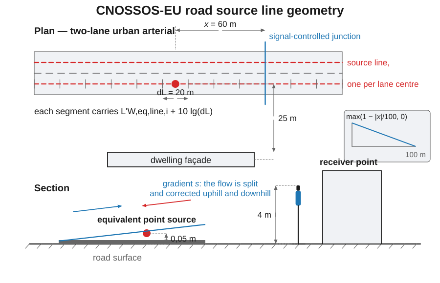
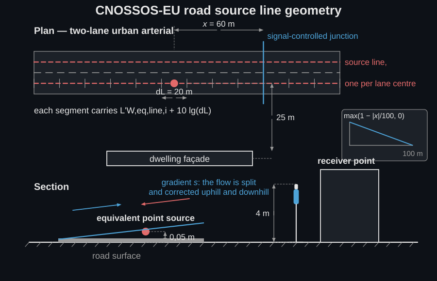
Section titled “2. The source and the source line”Each vehicle is one point source 0,05 m above the road surface, radiating uniformly; the first reflection on the pavement is already inside the sound power, which is why the method calls it a semi-free-field quantity. A traffic flow is an incoherent source line, ideally one line per lane at the lane centre.
For each vehicle category and octave band , formula (2.2.1) turns a single-vehicle sound power into a power per metre of line:
with in vehicles per hour and in km/h. The vehicle power itself is the energy sum of a rolling and a propulsion term (2.2.2), except for the powered two-wheelers of category 4, which have no rolling noise at all and take the propulsion term alone (2.2.3):
Table [2.2.a] defines five vehicle categories: 1 light motor vehicles, 2 medium heavy vehicles, 3 heavy vehicles, 4 powered two-wheelers and 5 the “open” category reserved for vehicle types not yet defined. Category 4 splits into the subclasses 4a mopeds and 4b motorcycles, which operate in very different driving modes, so the coefficient database carries five rows: 1, 2, 3, 4a and 4b. The first four categories are mandatory and category 5 is optional; it has no coefficients in Appendix F and is not modelled here.
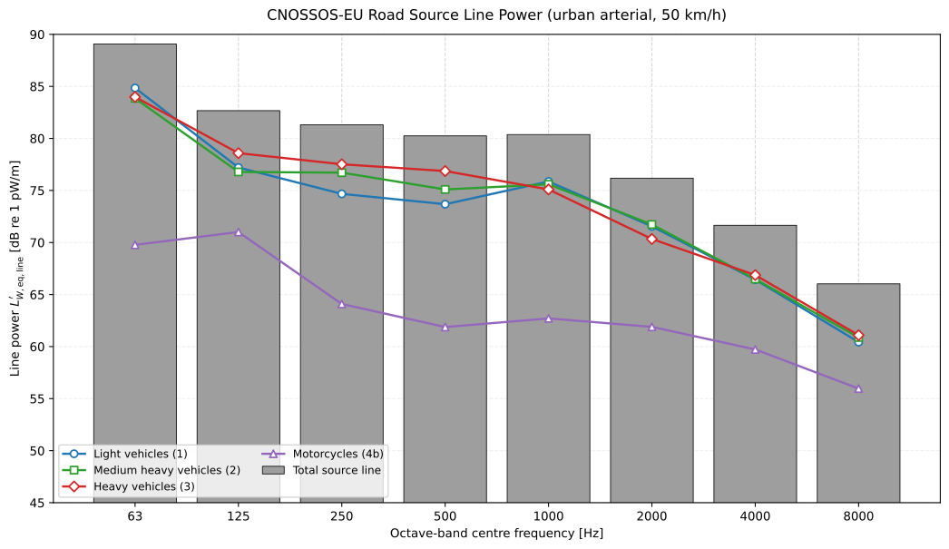
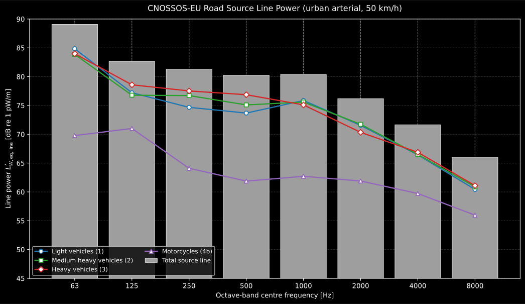
Light vehicles carry the flow, but 45 heavy vehicles per hour still take over the mid frequencies: the per-metre spectrum shows exactly where each category governs.
Show the code for this figure
import matplotlib.pyplot as pltfrom phonometry import environment
traffic = [    environment.RoadTraffic(environment.RoadVehicleCategory.LIGHT, 1200.0, 50.0),    environment.RoadTraffic(environment.RoadVehicleCategory.MEDIUM_HEAVY, 90.0, 50.0),    environment.RoadTraffic(environment.RoadVehicleCategory.HEAVY, 45.0, 50.0),    environment.RoadTraffic(environment.RoadVehicleCategory.MOTORCYCLES, 60.0, 50.0),]result = environment.road_source_power(    traffic, surface=environment.RoadSurface.THIN_LAYER_A, temperature_c=12.0, road_slope_percent=3.0,    junction_distance=60.0, junction_type=environment.JunctionType.CROSSING,)print(result.total_line_power.round(1))# [89.1 82.7 81.3 80.2 80.4 76.2 71.7 66. ]  dB re 1 pW per metre of lineprint(round(float(result.a_weighted_line_power), 1))     # 84.2 dB(A) per metreresult.plot()plt.show()
What a road source is worth. This urban arterial (1 200 light, 90 medium
heavy, 45 heavy vehicles and 60 motorcycles per hour at 50 km/h) comes out at
84,2 dB(A) per metre of line; the free-flowing motorway link of section 6
(1 000 light and 120 heavy vehicles per hour at 90 and 80 km/h) reaches
88,6 dB(A) per metre. Those are the two magnitudes to check your own result
against. The arithmetic behind them is worth holding on to: doubling the flow
adds exactly 3 dB, while halving the speed adds 3 dB to the flow term
and subtracts from the rolling term, so the two partly
cancel and an urban link is only a few decibels below a motorway one. The
spectrum says which mechanism is in charge: the motorway peaks at 1 kHz because
rolling noise leads, the arterial peaks at 63 Hz and stays flatter, because at
50 km/h with heavy vehicles and a junction 60 m away the propulsion term has
taken over. The check a reader can run on either: a_weighted_line_power must
equal the A-weighted energy sum of the printed band values, using the octave-band
CNOSSOS_A_WEIGHTING of section 6.
Where each input comes from
Section titled “Where each input comes from”Every argument of road_source_power is a defined quantity in Annex II, and
getting one wrong is a silent error: the call succeeds and the map is off by
decibels. This is where each of them is read from.
| Argument | What it means | Where it is read from | The trap |
|---|---|---|---|
RoadTraffic.flow_rate () | Vehicles of category per hour | Yearly average per hour, per time period (day / evening / night), per vehicle class and per source line, from traffic counting or a traffic model (2.2.1) | A peak-hour count. is an annual average for the period, which is what makes the result an ingredient |
RoadTraffic.speed () | Representative speed of category | In most cases the lower of the legal maximum for the road section and the legal maximum for the vehicle category; where local measurement data is unavailable, the legal maximum for the category (2.2.1) | Assuming a measured average is required. It is not: the standard’s default is the legal limit, and heavy vehicles usually take a lower one than the section |
temperature_c () | Air temperature | The yearly average air temperature of the period, from long-term meteorological data (2.2.10) | The survey-day value. At dB/°C, a 12 °C annual mean against a 20 °C afternoon is 0,6 dB on the light-vehicle rolling term |
RoadTraffic.studded_fraction, studded_months (, ) | Fleet share and season | The average ratio of light vehicles per hour fitted with studded tyres during the months they are fitted, and the number of those months; the method forms itself (2.2.7) | Passing the year-averaged share, which applies twice |
junction_distance () | Distance to the junction | Measured along the road from the point source to the nearest intersection of this source line with another source line (2.2.5) | Measuring to the stop line or the kerb. It is the line crossing, and only the last 100 m is affected |
junction_type () | 1 crossing with lights, 2 roundabout | The junction control, not its shape | A priority junction is neither: the correction is defined for signals and roundabouts |
road_slope_percent () | Signed longitudinal slope, % | The terrain model along the source line, saturating at ±12 % | Applying one sign to a two-way flow. The standard requires splitting the flow in half and correcting one half uphill and the other downhill |
surface | Pavement type | The road register, matched to a Table F-4 row and its declared speed range | Using a row outside its validity range |
| geometry | Source line and receiver | One line per lane at the lane centre (one line per carriageway, or one for a two-way road, is also acceptable), the point source 0,05 m above the surface; the Directive’s receiver points are 4 m above ground | Placing the source at the kerb, or at a vehicle-body height |
Two consequences worth stating outright. First, the temperature has to belong to the same period as and : a night flow paired with an annual mean temperature and a night speed is what makes the resulting line power an ingredient rather than a snapshot of one evening. Second, the source line is a modelling object, not a lane marking: moving it from the lane centre to the kerb changes every propagation distance downstream of it.
3. Rolling noise (2.2.4 to 2.2.10)
Section titled “3. Rolling noise (2.2.4 to 2.2.10)”Rolling noise is tyre-road noise. It grows logarithmically with speed from the reference speed :
where the correction collects four independent effects (2.2.5): the road surface, the studded tyres, the junction and the air temperature.
Air temperature (2.2.10) is a straight line, applied equally to all eight bands: , with for light vehicles and for the two heavy categories. Cold air makes tyres harder and the road louder, so the correction is positive below 20 °C.
Studded tyres (2.2.6 to 2.2.9) apply to category 1 only. The per-tyre excess saturates below 50 km/h and above 90 km/h, and the fleet-level correction weights it by the share of the year that studded tyres are on the road, :
Junctions (2.2.17, 2.2.18) add the same linear taper to both terms: for rolling noise and for propulsion noise, with the distance in metres from the point source to the nearest intersection of its source line with another source line, and the junction type: 1 for a crossing with traffic lights, 2 for a roundabout. Both are attributed equally to all octave bands. The rolling coefficients are negative (traffic near a junction is slower), the propulsion coefficients positive (it is accelerating), and the standard states explicitly that both are zero from m.
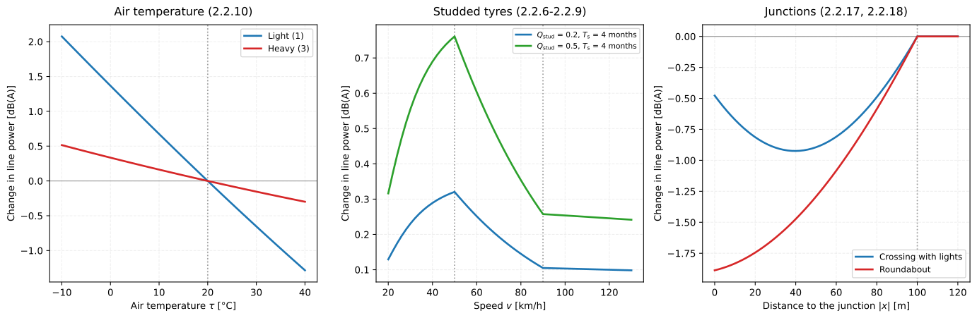
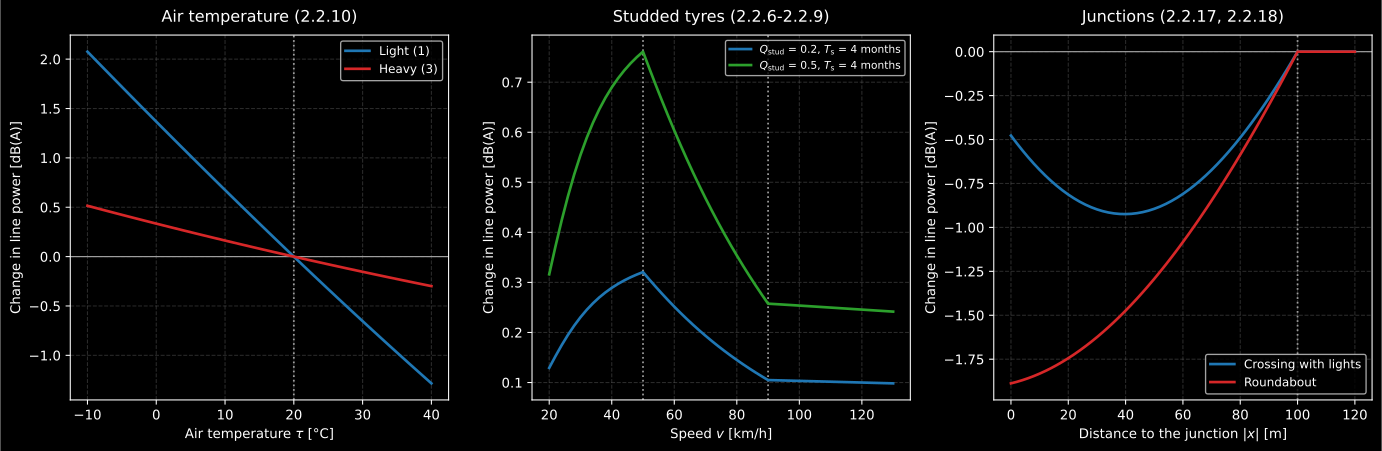
The three corrections of this section, each drawn as what it actually does to the line power. The temperature term is the only one that is exactly linear and the only one that changes sign; the studded term is a saturating band between 50 and 90 km/h; and the junction term is not monotone, because the negative rolling coefficient and the positive propulsion coefficient taper together. For a crossing the deepest reduction is around 50 m, not at the junction.
Show the code for this figure
import matplotlib.pyplot as pltimport numpy as np
# `road_source_power`, `RoadTraffic`, `RoadVehicleCategory` and `JunctionType`# are imported by the figure snippet above.def a_line(**kwargs):    return float(environment.road_source_power(**kwargs).a_weighted_line_power)
light = [environment.RoadTraffic(environment.RoadVehicleCategory.LIGHT, 1000.0, 50.0)]heavy = [environment.RoadTraffic(environment.RoadVehicleCategory.HEAVY, 1000.0, 50.0)]temps = np.linspace(-10.0, 40.0, 60)fig, (t_ax, s_ax, j_ax) = plt.subplots(1, 3, figsize=(13, 4.2))for flow, name in [(light, "Light (1)"), (heavy, "Heavy (3)")]:    ref = a_line(traffic=flow)    t_ax.plot(temps, [a_line(traffic=flow, temperature_c=t) - ref for t in temps],              label=name)t_ax.set(xlabel="Air temperature tau [°C]", ylabel="Change in line power [dB(A)]")t_ax.legend()
speeds = np.linspace(20.0, 130.0, 60)for share in (0.2, 0.5):    s_ax.plot(speeds, [        a_line(traffic=[environment.RoadTraffic(environment.RoadVehicleCategory.LIGHT, 1000.0, v,                                                studded_fraction=share)],               studded_months=4.0)        - a_line(traffic=[environment.RoadTraffic(environment.RoadVehicleCategory.LIGHT, 1000.0, v)])        for v in speeds], label=f"Qstud,ratio = {share:g}, Ts = 4 months")s_ax.set(xlabel="Speed v [km/h]", ylabel="Change in line power [dB(A)]")s_ax.legend(fontsize="small")
xs = np.linspace(0.0, 120.0, 60)ref = a_line(traffic=light)for junction, name in [(environment.JunctionType.CROSSING, "Crossing with lights"),                       (environment.JunctionType.ROUNDABOUT, "Roundabout")]:    j_ax.plot(xs, [a_line(traffic=light, junction_distance=float(x),                          junction_type=junction) - ref for x in xs], label=name)j_ax.set(xlabel="Distance to the junction |x| [m]",         ylabel="Change in line power [dB(A)]")j_ax.legend(fontsize="small")plt.show()
4. Propulsion noise (2.2.11 to 2.2.16)
Section titled “4. Propulsion noise (2.2.11 to 2.2.16)”Propulsion noise is the power train: engine, exhaust, transmission, intake. It is linear in speed, not logarithmic, because at low speed the engine is working hardest relative to the distance covered:
Where the two speed laws cross is what makes the road source behave the way it does: below the crossover the source is an engine, above it a tyre.
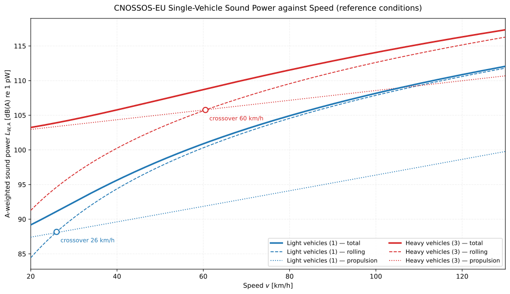
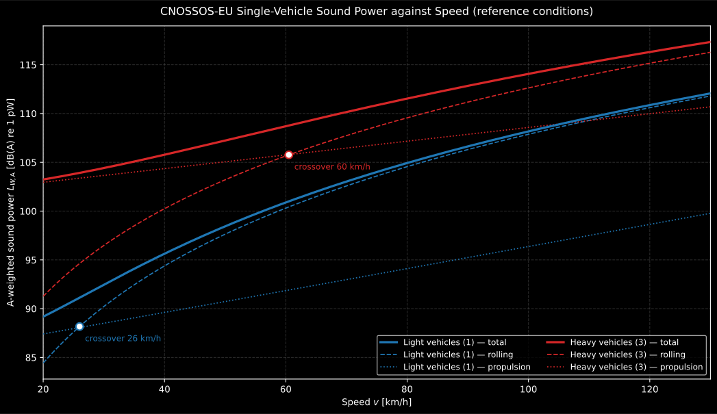
A light vehicle is tyre-dominated from about 25 km/h; a heavy vehicle only from about 60 km/h, which is why a lorry is still an engine at urban speeds.
Show the code for this figure
import matplotlib.pyplot as pltimport numpy as npfrom phonometry import environment
weights = np.asarray(environment.CNOSSOS_A_WEIGHTING)a_weighted = lambda bands: 10.0 * np.log10(np.sum(10.0 ** ((bands + weights) / 10.0)))
speeds = np.linspace(20.0, 130.0, 221)fig, ax = plt.subplots()for category, name in [("1", "Light vehicles (1)"), ("3", "Heavy vehicles (3)")]:    rolling = [a_weighted(environment.road_rolling_noise(category, v)) for v in speeds]    propulsion = [a_weighted(environment.road_propulsion_noise(category, v)) for v in speeds]    total = [a_weighted(environment.road_vehicle_sound_power(category, v)) for v in speeds]    ax.plot(speeds, total, lw=2.4, label=f"{name} - total")    ax.plot(speeds, rolling, ls="--", lw=1.2, label=f"{name} - rolling")    ax.plot(speeds, propulsion, ls=":", lw=1.2, label=f"{name} - propulsion")ax.set_xlabel("Speed v [km/h]")ax.set_ylabel("A-weighted sound power [dB(A) re 1 pW]")ax.legend(fontsize="small")plt.show()
Road gradient (2.2.13 to 2.2.16) is the one correction whose published form is genuinely asymmetric, and the asymmetry is not a transcription slip. For light vehicles the downhill branch has no speed factor, while the two heavy categories do and use different speed offsets:
| Category | Downhill ( below the breakpoint) | Flat band | Uphill |
|---|---|---|---|
| 1 | −6 % to 2 % | ||
| 2 | −4 % to 0 % | ||
| 3 | −4 % to 0 % |
Category 4 takes no gradient correction. The slope saturates at 12 % in both directions. Downhill noise comes from engine braking, uphill noise from load, so both branches are positive. For a bidirectional flow, split the flow in two and correct one half uphill and the other downhill.
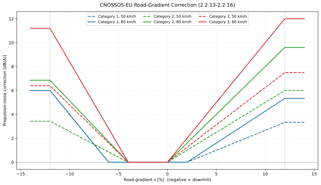
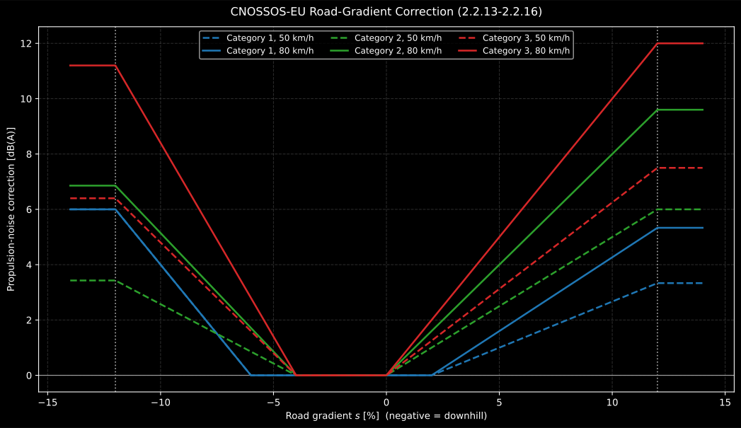
The asymmetry is a shape, not a typo. Each category has its own flat band (−6 % to +2 % for light vehicles, −4 % to 0 % for the two heavy classes), each saturates at ±12 %, and both branches rise: downhill the engine brakes, uphill it works. At 80 km/h a 14 % descent is worth 6.0 dB(A) to a light vehicle and 11.2 dB(A) to a heavy one, while the same climb is worth 5.3 and 12.0 dB(A), and the light-vehicle downhill branch is the only one of the six that does not scale with speed.
Show the code for this figure
import matplotlib.pyplot as pltimport numpy as np
# `road_propulsion_noise` and `CNOSSOS_A_WEIGHTING` are imported by the# speed-law figure snippet above.weights = np.asarray(environment.CNOSSOS_A_WEIGHTING)a_weighted = lambda bands: 10.0 * np.log10(np.sum(10.0 ** ((bands + weights) / 10.0)))
slopes = np.linspace(-14.0, 14.0, 141)fig, ax = plt.subplots()for category in ("1", "2", "3"):    for speed, style in [(50.0, "--"), (80.0, "-")]:        flat = a_weighted(environment.road_propulsion_noise(category, speed))        ax.plot(slopes,                [a_weighted(environment.road_propulsion_noise(category, speed, road_slope_percent=s)) - flat                 for s in slopes], style, label=f"Category {category}, {speed:g} km/h")ax.set_xlabel("Road road_slope_percent s [%]")ax.set_ylabel("Propulsion-noise correction [dB(A)]")ax.legend(fontsize="small")plt.show()
Below 20 km/h the vehicle stops getting quieter. Clause 2.2.1 states, after
both (2.2.2) and (2.2.3), that for speeds under 20 km/h the sound power takes its
20 km/h value: the tabulated regressions were fitted to free-flowing traffic and
are not extrapolated into a queue. The flow term keeps the true speed, so the
two halves of (2.2.1) pull in opposite directions and the line power has a
minimum. For 1 000 light vehicles per hour on the reference surface,
road_source_power returns 81,5 dB(A) per metre at 50 km/h, 76,2 at 20 km/h,
79,2 at 10 km/h and 82,2 at 5 km/h; the same road gets louder per metre as the
stream slows below the floor, purely because more vehicles are on each metre of
it. A reader who does not know the floor cannot tell that from a modelled
congestion effect.
Say what the model therefore does not represent: acceleration and braking cycles, idling in a queue, and the propulsion noise of stop-start driving, for which the junction correction over the last 100 m is a deliberate crude proxy. Congested links are normally modelled at their average travel speed with that correction applied.
5. The road surface (2.2.19, 2.2.20 and Table F-4)
Section titled “5. The road surface (2.2.19, 2.2.20 and Table F-4)”Table F-4 gives, for the reference surface and each of fourteen named pavements, an octave-band coefficient and a speed coefficient , per vehicle category, with the speed range over which the row is declared valid. The surface enters the two terms differently:
An absorbing surface reduces propulsion noise; a noisy one does not increase it. That asymmetry is deliberate: the pavement can absorb the engine sound radiated down onto it, but a rough texture only generates tyre noise, and tyre noise is already the rolling term.
from phonometry import environment
row = environment.road_surface_coefficients(environment.RoadSurface.TWO_LAYER_ZOAB_FINE)row.speed_range          # (80.0, 130.0) km/h, the printed validity rangerow.alpha["1"]           # alpha per octave band for light vehiclesrow.beta["1"]            # -0.1, the speed coefficient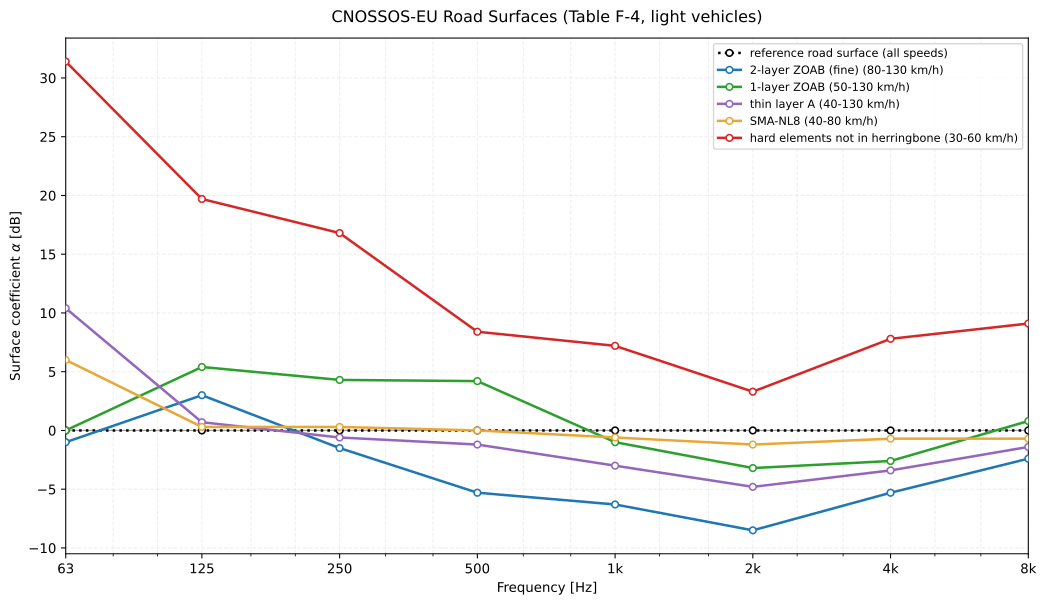
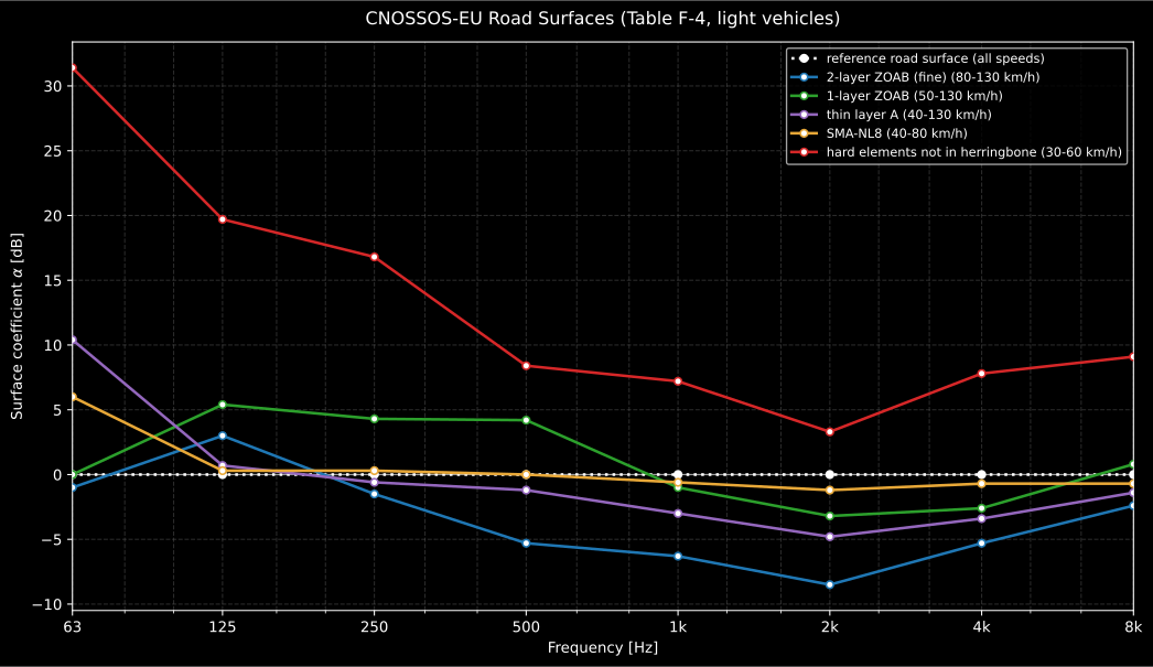
The reference surface is the zero line, so every curve reads directly as “louder or quieter than the CNOSSOS reference”: the two-layer porous asphalt is 6,3 dB below it at 1 kHz, hard elements not laid in herringbone are 31,4 dB above it at 63 Hz. The declared speed range in the legend is part of the row: a porous asphalt validated from 80 to 130 km/h is not a coefficient set for a 30 km/h street, the reference row alone carries no range, and the method offers no interpolation between rows.
Show the code for this figure
import matplotlib.pyplot as pltimport numpy as np
# `RoadSurface` and `road_surface_coefficients` are imported just above.bands = np.array([63.0, 125.0, 250.0, 500.0, 1000.0, 2000.0, 4000.0, 8000.0])fig, ax = plt.subplots()for surface in (environment.RoadSurface.REFERENCE, environment.RoadSurface.TWO_LAYER_ZOAB_FINE,                environment.RoadSurface.ONE_LAYER_ZOAB, environment.RoadSurface.THIN_LAYER_A,                environment.RoadSurface.SMA_NL8, environment.RoadSurface.HARD_ELEMENTS_NOT_HERRINGBONE):    row = environment.road_surface_coefficients(surface)    # The reference row carries no speed range: it is valid by definition.    span = ("all speeds" if row.speed_range is None            else "{:g}-{:g} km/h".format(*row.speed_range))    ax.semilogx(bands, row.alpha["1"], label=f"{surface.value} ({span})")ax.axhline(0.0, color="k", lw=0.8)ax.set_xlabel("Octave-band centre frequency [Hz]")ax.set_ylabel("Surface coefficient alpha, category 1 [dB]")ax.legend(fontsize="small")plt.show()
The reference surface of the first row is all zeros: it is the virtual average of a dense asphalt concrete 0/11 and a stone mastic asphalt 0/11, between two and seven years old, in representative maintenance condition, dry, with no studded tyres, at 20 °C, on the flat. Under exactly those conditions every correction in 2.2 vanishes identically, so at the reference speed , where the two speed terms vanish as well, the sound powers are the Table F-1 coefficients and .
6. Handing the source to a propagation model
Section titled “6. Handing the source to a propagation model”The emission stage produces a power per metre. Splitting that line into equivalent point sources is, in the words of section 2.5.3, “outside the scope of the current methodology”: a point source standing for a segment of length simply carries , which is arithmetic and is offered as such.
import numpy as npfrom phonometry import environment
result = environment.road_source_power([    environment.RoadTraffic(environment.RoadVehicleCategory.LIGHT, 1000.0, 90.0),    environment.RoadTraffic(environment.RoadVehicleCategory.HEAVY, 120.0, 80.0),])segment = environment.line_source_segment_power(result.total_line_power, 20.0)  # a 20 m segment
# One segment, the one directly opposite a receiver 100 m from the road.levels = environment.predicted_receiver_level(    segment,    environment.PropagationGeometry(100.0, result.source_height, 4.0),    frequencies=result.frequencies,)
# The road is the energy sum of its segments: 1 km either way, in 20 m steps.energy = np.zeros_like(levels)for x in np.arange(-990.0, 1000.0, 20.0):        # segment centres along the road    energy += 10 ** (environment.predicted_receiver_level(        segment,        environment.PropagationGeometry(float(np.hypot(100.0, x)), result.source_height, 4.0),        frequencies=result.frequencies,    ) / 10)road = 10 * np.log10(energy)
Two rules make a segmentation defensible, and neither is method: 2.5.3 declares the split out of scope, so this is engineering practice. Each segment must be short enough that the point source at its centre stands for the whole segment. ISO 9613-2 allows one equivalent point source only where the propagation distance exceeds twice the largest source dimension, so a segment seen from 100 m may be tens of metres long while one seen from 10 m may not. And the road must be modelled far enough in both directions that the tails stop mattering: beyond roughly ten times the perpendicular offset, adding segments changes the total by less than a tenth of a decibel, which is why 1 km either way is enough at 100 m here. The two spectra are read out in dB(A) two paragraphs down: 52.9 dB(A) for the single segment against 64.7 dB(A) for the road, an 11.8 dB difference that is entirely the arithmetic above.
Note what this is and is not. CNOSSOS-EU has its own propagation method in section 2.5 of Annex II, and it is not ISO 9613-2: the two differ in the ground model, in the diffraction treatment and in the way favourable and homogeneous conditions are combined. Chaining a CNOSSOS emission onto the ISO 9613-2 propagation of this library is a legitimate engineering estimate, but it is not the normative CNOSSOS chain and must not be reported as one.
For the A-weighted total, use the octave-band weighting the Directive itself prints in 2.5.5 as amended, rather than recomputing it:
from phonometry import environment
environment.CNOSSOS_A_WEIGHTING   # (-26.2, -16.1, -8.6, -3.2, 0.0, 1.2, 1.0, -1.1)result.a_weighted_line_power
# The two receiver spectra of the segmentation above, A-weighted:weight = np.asarray(environment.CNOSSOS_A_WEIGHTING)print(round(float(10 * np.log10(np.sum(10 ** ((levels + weight) / 10)))), 1))# 52.9 dB(A) - one 20 m segment, not the roadprint(round(float(10 * np.log10(np.sum(10 ** ((road + weight) / 10)))), 1))# 64.7 dB(A) - the same road, summed over 2 km: 11.8 dB more
7. Substituting a national database
Section titled “7. Substituting a national database”Appendix F is called a database, not a table of constants, because Member States may substitute measured national values, and because the same equations have already been evaluated with two different coefficient sets (the 2015 one and the 2021 one). Both coefficient objects can be replaced:
import dataclasses
from phonometry import environment
# One measured national row for light vehicles, the rest of Appendix F as published.national = dataclasses.replace(    environment.ROAD_COEFFICIENTS,    rolling_a={        **environment.ROAD_COEFFICIENTS.rolling_a,        "1": (83.4, 89.0, 88.1, 93.6, 100.4, 96.9, 87.0, 76.5),    },)
A substituted database has to cover every category of the traffic it is used
with: reaching for a category it does not carry raises ValueError rather than
failing later.
That mechanism is also what pins the implementation: the European Commission published a test set of 4 875 road emission cases computed with the 2015 coefficients, and feeding the shipped equations that superseded database (not the 2021 tables the library ships by default) reproduces every published band level to 0,005 dB, inside the two decimals the test set prints.
What this guide covers
Section titled “What this guide covers”Covered
Section 2.2 of Annex II to Directive 2002/49/EC in the consolidated text: the traffic-flow line power (2.2.1), the vehicle power (2.2.2, 2.2.3), rolling noise with its studded-tyre and temperature corrections (2.2.4 to 2.2.10), propulsion noise with the road-gradient correction (2.2.11 to 2.2.16), the junction correction (2.2.17, 2.2.18) and the road-surface effect (2.2.19, 2.2.20), together with the whole Appendix F database, through
road_source_power,road_vehicle_sound_power,road_rolling_noise,road_propulsion_noiseandroad_surface_coefficients.Not covered
The railway source (2.3 and Appendix G), the industrial source (2.4 and Appendix H), the aircraft source (2.6 and 2.7) and the CNOSSOS-EU propagation method of section 2.5, which is a different model from the ISO 9613-2 one implemented in this library. The open vehicle category 5 has no coefficients in Appendix F and is therefore not modelled. How a source line is split into point sources is declared out of scope by the method itself.
References
Section titled “References”- European Union. (2015). Commission Directive (EU) 2015/996 establishing common noise assessment methods according to Directive 2002/49/EC of the European Parliament and of the Council (Directive (EU) 2015/996). Replaces Annex II of Directive 2002/49/EC with the CNOSSOS-EU methods. The implemented road source is section 2.2 (formulae 2.2.1 to 2.2.20) with the coefficient database of Appendix F.
- European Union. (2018). Corrigendum to Commission Directive (EU) 2015/996 (OJ L 5, 10.1.2018, p. 35). Corrects the octave-band range of the road source to 63 Hz - 8 kHz, replaces the whole of Appendix G and fixes the railway roughness conversion to metres per second.
- European Union. (2021). Commission Delegated Directive (EU) 2021/1226 amending, for the purposes of adapting to scientific and technical progress, Annex II to Directive 2002/49/EC as regards common assessment methods for noise (Directive (EU) 2021/1226). The amendment in force since 31 December 2021. Replaces Tables F-1 and F-4 in their entirety and prints the octave-band A-weighting used to sum the source spectrum.
- International Organization for Standardization. (1996). Acoustics — Attenuation of sound during propagation outdoors — Part 2: General method of calculation (ISO 9613-2:1996). The propagation model used here to carry the emission to a receiver. CNOSSOS-EU has its own propagation method in section 2.5 of Annex II, which is not ISO 9613-2.
- Kephalopoulos, S., Paviotti, M., & Anfosso-Lédée, F. (2012). Common noise assessment methods in Europe (CNOSSOS-EU) (EUR 25379 EN). Publications Office of the European Union. https://doi.org/10.2788/31776The Joint Research Centre reference report the Directive text descends from, with the measurement campaigns behind the Appendix F coefficients.