Soundscape Analysis (ISO/TS 12913)
Standards: ISO/TS 12913ISO 12913
A sound level tells how much sound arrives at a place. It does not tell whether the people there find it pleasant, busy, calming or annoying, and two squares at the same can be heard as opposite places. A soundscape is the acoustic environment as a person perceives it, in context (ISO 12913-1), and its study “relies primarily upon human perception and only then turns to physical measurement” (ISO/TS 12913-2).
That makes this the first page of the library whose input is not a signal but a questionnaire: the boxes people ticked on a soundwalk. ISO/TS 12913-2 prints the questionnaires and says what a study has to report; ISO/TS 12913-3 turns the ticks into numbers, places each site on a two-dimensional model of how pleasant and how eventful it sounds, correlates the answers with the acoustic measurements, and says how a binaural recording made at the same place is analysed.
This page implements the 2019 edition of ISO/TS 12913-3. ISO has published a 2025 edition that revises Annex A, where the pleasantness and eventfulness formulas are; it has not been read for this implementation, so a study that cites the 2025 edition should check those formulas against it.
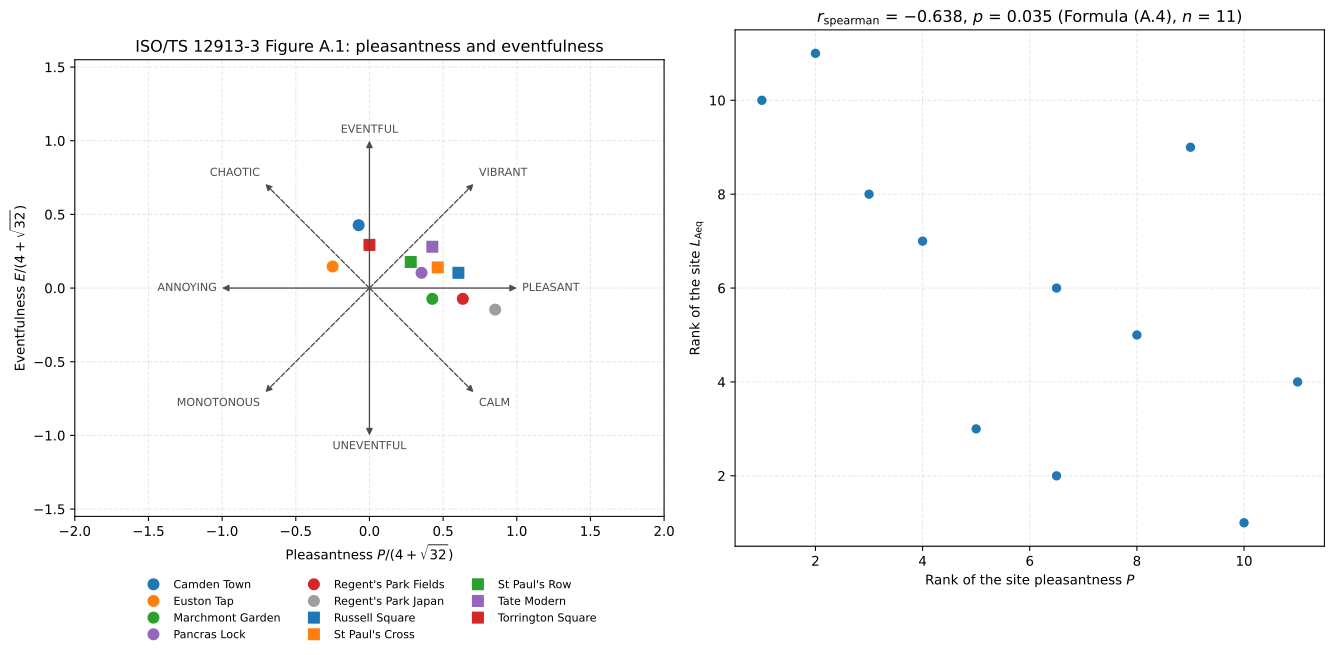
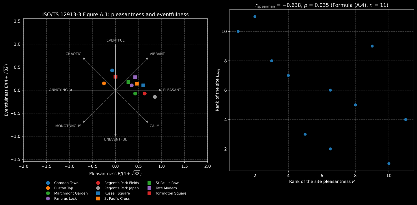
Eleven London sites of the International Soundscape Database on the model of
Figure A.1 (left), and the rank correlation of their pleasantness with their
level (right), both drawn by the results’ own .plot(), with the two rank
axes named for what was ranked.
1. The questionnaire and its scale values
Section titled “1. The questionnaire and its scale values”Method A of ISO/TS 12913-2 (clause C.3.1) is a questionnaire in four parts, every one on five boxes: which sources are heard and how much (Figure C.2, or the three-source Figure C.3), how the place is perceived on eight attributes (Figure C.4), how good the sound environment is overall (Figure C.5) and how appropriate it is to the place (Figure C.6). The library publishes all of it, every question, item and response category as printed, with the scale values ISO/TS 12913-3 Table A.1 assigns:
from phonometry import environment
part2 = environment.METHOD_A_SCALES[2]print(part2.figure, part2.categories[0], part2.scale_values)  # C.4 Strongly agree (5, 4, 3, 2, 1)print(environment.method_a_scale_values([1, 2, 5], part=2))  # [5. 4. 1.]print(environment.method_a_scale_values([1, 2, 5], part=4))  # [1. 2. 5.]
The orientation is the thing to get right. Parts 1 and 4 run 1 to 5 from the
left-hand box, so “not at all” is 1; parts 2 and 3 run 5 to 1, so
“strongly agree” and “very good” are 5. method_a_scale_values converts the
position of a ticked box, counted from the left, into the value of its part;
everything after it takes scale values, never box positions.
The tables keep the text as printed, including two slips of the page: the questions of Figures C.2 to C.4 read “to what extend” and their instructions “reponse alternative”. A study that prints its questionnaire from them should correct both; the errata register has the entry.
2. Median and range per site
Section titled “2. Median and range per site”Every Method A scale is ordinal, so ISO/TS 12913-3 A.2 reports the median of each item per site as its central tendency and the range as its dispersion. A blank answer is left out of both:
answers = {"pleasant": [5, 4, 4, 2, 5], "annoying": [1, 2, 1, 4, 1]}summary = environment.method_a_summary( answers, part=2, sites=["park", "park", "park", "road", "road"])print(summary.sites) # ('park', 'road')print(summary.medians.tolist()) # [[4.0, 1.0], [3.5, 2.5]]print(summary.ranges.tolist()) # [[1.0, 1.0], [3.0, 3.0]]A 2-D array (responses, items) is read in the order of the part’s figure,
and summary.plot() draws each item’s median with its range as a bar, site
beside site.
3. Pleasantness and eventfulness
Section titled “3. Pleasantness and eventfulness”The eight attributes of part 2 are not eight independent judgements. When people describe how an environment feels, their answers fall on two dimensions: how pleasant it is, and how eventful, how busy with human and other activity. Rotating those two axes by 45 degrees gives the other two pairs of attributes: vibrant is pleasant and eventful, chaotic eventful and annoying, monotonous annoying and uneventful, calm uneventful and pleasant. Formulas (A.1) and (A.2) project the eight answers onto the two main axes, with weighting the diagonal ones:
with pleasant, annoying, calm, chaotic, vibrant, monotonous, eventful and uneventful, each a scale value from 1 to 5. Every term is a difference, so a respondent who gives every attribute the same answer sits at the origin, and the extremes are : 4 from the main axis and from the two diagonals. Dividing by maps the coordinates to .
The eleven London sites of the International Soundscape Database were surveyed almost entirely with the English questionnaire of Method A; ten answers, at four of the sites, were given on the Spanish version of the database’s survey and are counted too. Here are the site medians of their answers and the median of their recordings:
sites = ["Camden Town", "Euston Tap", "Marchmont Garden", "Pancras Lock",         "Regent's Park Fields", "Regent's Park Japan", "Russell Square",         "St Paul's Cross", "St Paul's Row", "Tate Modern", "Torrington Square"]# Site medians of the eight attributes, in the order of Figure C.4:# pleasant, chaotic, vibrant, uneventful, calm, annoying, eventful, monotonous.medians = [    [3, 4, 4, 2, 2, 3, 4, 3], [2, 4, 3, 3, 2, 3, 3, 3], [4, 2, 3, 3, 4, 2, 3, 2],    [4, 3, 3, 2, 4, 2, 3, 2], [5, 2, 3, 3, 4, 1, 3, 2], [5, 1, 4, 3, 5, 1, 3, 2],    [4, 2, 4, 2, 4, 1, 3, 2], [4, 2.5, 4, 2, 4, 2, 3, 2], [4, 3, 4, 2, 3, 2, 3, 3],    [4, 3, 4, 2, 4, 2, 4, 2], [3, 4, 4, 3, 2, 3, 3, 2],]laeq_db = [69.96, 69.45, 55.14, 59.02, 53.12, 59.74, 66.12, 61.83, 63.34, 63.00, 63.51]
pe = environment.pleasantness_eventfulness(medians, sites=sites)print(round(pe.normalized_pleasantness[5], 2), round(pe.normalized_eventfulness[5], 2))  # 0.85 -0.15print(round(pe.normalized_pleasantness[0], 2), round(pe.normalized_eventfulness[0], 2))  # -0.07 0.43print(round(environment.PLEASANTNESS_EVENTFULNESS_RANGE, 2))  # 9.66
Regent’s Park Japanese Garden (index 5) comes out the most pleasant and
slightly uneventful, in the calm quadrant; Camden Town (index 0) is the most
eventful and a little on the annoying side. pe.plot() draws the model of
Figure A.1 with every site on it, the left panel of the figure at the top.
Given the answers of each respondent rather than site medians,
pleasantness_eventfulness returns both: every respondent’s own coordinates
(respondent_pleasantness, respondent_eventfulness) and the site’s. The site
point is the formulas applied to the site median of each attribute, since
A.2 makes the median the central tendency of the scale;
central_tendency="mean" uses the mean instead. When every respondent answered
all eight attributes, that mean point is also the mean of the respondents’
coordinates, the formulas being linear; a blank answer breaks the equality,
because each attribute mean then runs over the respondents who answered that
attribute. pe.plot(respondents=True) adds every respondent as a faint point
in the colour of their site.
Clause A.3 introduces the formulas as processing “the results from part 3”. The attributes they read are part 2, as Table A.1, the rest of Annex A and ISO/TS 12913-2 Figure C.4 all say; part 3 is the single overall rating of Figure C.5. The library applies them to part 2, and the errata register has the entry.
4. Linking the ratings to the acoustic data
Section titled “4. Linking the ratings to the acoustic data”A study then asks whether what people say goes with what was measured. For ordinal data A.4 prescribes Spearman’s rank correlation: without ties Formula (A.3),
with the difference of the ranks of pair , and with ties in either variable Formula (A.4), which corrects the rank variances by the tie sums and of the two variables and is Pearson’s coefficient of the average ranks. The site medians above have ties, so:
rho = environment.spearman_rank_correlation(pe.pleasantness, laeq_db)print(rho.formula, round(rho.coefficient, 3), round(rho.p_value, 3))  # (A.4) -0.638 0.035
r = environment.pearson_correlation(pe.pleasantness, laeq_db)print(r.formula, round(r.coefficient, 3), round(r.p_value, 3))  # (B.1) -0.66 0.027
Across these eleven sites the louder places are the less pleasant ones, and
significantly so. Over all 26 locations of the database the rank correlation
is about (). A.4 and B.3 ask for the probability value
without naming a test; both functions use the Student statistic
with degrees of freedom, exact for Pearson’s
coefficient of bivariate normal data and the usual approximation for
Spearman’s.
alternative="greater" or "less" gives the one-sided value.
Three details of the page are worth knowing. Formula (A.3) is printed as
, with a stray factor 1 that the library
reads as the typesetting remnant it is. The where-list under Formula (A.4)
defines as “the number of in tied ranks” and as “the numbers
of tied ranks”; the library reads them as the size of each group of tied values
and the number of those groups, the usual tie correction. And Formula (B.2),
Pearson’s covariance for interval data, divides by ; the standard deviations
of (B.1) are then taken with as well, which is what makes the usual
coefficient. The first two, and a stray capital in the where-list of (B.2), are
in the errata register.
rho.plot() draws the ranked pairs, the right panel of the figure at the top.
5. Method B: continuous scales and the source ranking
Section titled “5. Method B: continuous scales and the source ranking”Method B (ISO/TS 12913-2 C.3.2) is the soundwalk data collection: at each stop the participants mark continuous scales, list the sources they noticed from the most noticeable down, and write down what went through their mind. A mark may fall anywhere along a scale; its value runs from 1 at the left-hand tick to 5 at the right-hand one and is taken to one decimal (ISO/TS 12913-3 B.2). The level of measurement is interval, so B.2 reports the mean, the standard deviation and the 95 % confidence interval per site:
print(environment.method_b_scale_values([0.0, 0.37, 1.0]))  # [1.  2.5 5. ]
ratings = {"How loud is it here?": [3.9, 4.2, 3.1, 4.4, 3.6, 4.0]}b = environment.method_b_summary(ratings)print(round(b.means[0, 0], 2), round(b.standard_deviations[0, 0], 2))       # 3.87 0.46print(round(b.confidence_lower[0, 0], 2), round(b.confidence_upper[0, 0], 2))  # 3.38 4.35
ranking = environment.method_b_source_ranking(    [["traffic", "voices", "birds"], ["traffic", "birds"], ["voices", "traffic"], ["traffic"]])print(ranking.sources, ranking.median_ranks[0].tolist())  # ('traffic', 'voices', 'birds') [1.0, 1.5, 2.5]
The interval is the Student one about the mean with the sample standard deviation; the median is reported beside it, as the “statistics for an ordinal scale level” B.2 allows. The source ranking is ordinal too: the median rank of each source and its range, over the participants who listed it.
The text of C.3.2.3 describes three scales labelled from “not at all” to
“extremely”; Figure C.7 prints four, the fourth (“How often would you like to
visit this place again?”) labelled from “never” to “very often”.
METHOD_B_SCALES holds the four as printed and method_b_summary takes a
table of three or four of them; the contradiction is in the
errata register.
6. The binaural analysis
Section titled “6. The binaural analysis”A soundscape study records the place with an artificial head at 1.6 m, for at
least 3 min, sampled at 44.1 kHz or more (ISO/TS 12913-2 Annex D), and
equalizes the recording to approximate a monaural measurement before it is
analysed. Every metric of ISO/TS 12913-3 Table D.1 is then determined for
each ear, and the higher of the two is the single representative value
“indicating the overall experience”; their mean may be reported as well (D.2).
binaural_indicators does that for a calibrated two-channel recording, left
ear first, with the library’s own implementation of each metric. A synthetic
street, eight seconds with one vehicle passing left to right:
import warnings
import numpy as np
fs = 48_000rng = np.random.default_rng(12913)t = np.arange(8 * fs) / fsbackground = 0.02 * rng.standard_normal(t.size)swell = np.exp(-0.5 * ((t - 4.0) / 0.9) ** 2)vehicle = 0.08 * rng.standard_normal(t.size)left = background + swell * vehicleright = 0.9 * background + 10 ** (-3 / 20) * np.roll(swell, int(0.3 * fs)) * vehicle
with warnings.catch_warnings():    # Eight seconds is short of the 3 min of ISO/TS 12913-2 D.3, which the    # analysis would otherwise say with a SoundscapeWarning.    warnings.simplefilter("ignore", environment.SoundscapeWarning)    bi = environment.binaural_indicators(        np.vstack([left, right]), fs, parameters=("sound_pressure_level", "loudness", "sharpness")    )laeq = bi.metrics["LAeq,T"]print(round(laeq.left, 1), round(laeq.right, 1), round(laeq.representative, 1))  # 63.5 61.1 63.5print(round(bi.representative("N5"), 1), round(bi.representative("N5/N95"), 2))  # 22.2 2.27print(sorted(bi.not_implemented))  # ['S5', 'S95', 'Saverage']
Each row of the table comes from a function the library already has, and each
metric says which in its method:
| Table D.1 row | Metrics per ear | Computed with |
|---|---|---|
| Sound pressure level (ISO 1996-1) | , , , | signals.laeq, signals.leq of the C-weighted signal, signals.ln_levels with time weighting F |
| Loudness (ISO 532-1) | , , , , | psychoacoustics.loudness_zwicker, time-varying |
| Sharpness (DIN 45692) | , , | not computed, see below |
| Psychoacoustic tonality (ECMA 74) | psychoacoustics.tonality_ecma (ECMA-418-2:2025) | |
| Roughness | , | psychoacoustics.roughness_ecma (ECMA-418-2:2025) |
| Fluctuation strength | , | psychoacoustics.fluctuation_strength_ecma (ECMA-418-2:2025) |
is the root mean cube of the loudness over time, the cube
root of the mean of , as the formula of the NOTE under ISO/TS 12913-2
A.3 f) prints it; the text of that NOTE calls the second step “the exponent 3”
where the formula applies , and the
errata register has the entry. is
the variability ratio D.2 suggests. Table D.1 cites ECMA-74 for tonality; the
current edition of ECMA-74 refers its psychoacoustic tonality method to
ECMA-418-2 clause 6, which is what tonality_ecma implements. For roughness
and fluctuation strength the table cites a textbook, and ISO/TS 12913-2
Annex B noted in 2018 that no standardized method existed; the library uses the
hearing model of ECMA-418-2:2025 for both, and is the value that
model reports as its roughness (the value exceeded 10 % of the time).
The sharpness row is left empty, on purpose. ,
and are percentiles of a sharpness that varies in time. The library’s
DIN 45692 sharpness is computed from the stationary specific loudness, and its
time-varying loudness does not publish the specific loudness over time a
time-varying sharpness needs, so not_implemented says why instead of a
stationary number appearing under a percentile’s name.
The hearing-model metrics are expensive: on a 3 min recording tonality,
roughness and fluctuation strength take minutes each, tonality most of all.
parameters picks the rows to compute. A recording shorter than 3 min or
sampled below 44.1 kHz raises a SoundscapeWarning; the equalization, the
position and the calibration are the caller’s.
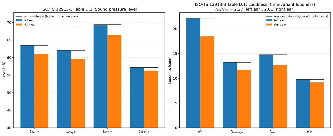
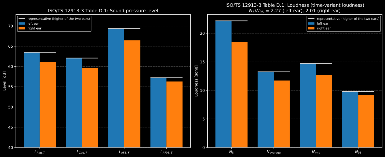
Two rows of Table D.1 at both ears of the synthetic street, from
bi.plot(parameter="sound_pressure_level") and bi.plot(parameter="loudness").
The left ear hears the vehicle first and louder, so it is the representative
ear for every metric.
7. What the report has to say
Section titled “7. What the report has to say”ISO/TS 12913-2 Annex A (normative) lists the minimum a soundscape study
reports: who the participants were and how they were selected (A.2), the
acoustic environment with the results of its measurements (A.3), and how the
perception data were collected (A.4), with a copy of the questionnaire.
SoundscapeReport holds the three records and refuses to be built with a
required item missing, naming its clause; the seven results of A.3 f) come
straight from the binaural analysis:
report = environment.SoundscapeReport( participants=environment.SoundscapeParticipants( selection="visitors approached at the entrance, one in three", residents_or_visitors="visitors", lay_or_expert="lay people", age_and_gender_distribution="18 to 74 years, 52 % women", other_relevant_information="self-reported normal hearing", ), acoustic_environment=environment.SoundscapeAcousticEnvironment( environment_type="real", sound_sources="road traffic in the background, a passing car in the foreground", weather_and_wind="dry, wind under 2 m/s", time_of_year_and_day="June, 14:00 to 16:00", measurement_points="kerbside, artificial head at 1.6 m facing the road", measurement_results=bi.reporting_results(), site_description="urban street, residential", ), data_collection=environment.SoundscapeDataCollection( methods="Method A questionnaire, parts 1 to 4", questions="Figures C.2 to C.6 of ISO/TS 12913-2, answers on paper", language="English, as printed in Annex C", instrument_copy="Appendix B", rating_scale_construction="five-category scales of Figures C.2 to C.6", ),)print(round(report.acoustic_environment.measurement_results["N5"], 1)) # 22.2Each item is free text, because the annex says what is stated and not how. A site description is required for a field study or recordings, the recording and reproduction for a recorded or virtual environment; a record that exists meets the minimum as far as a record can tell, and whether what it says is true and sufficient stays with the author.
Show the code for these figures
import matplotlib.pyplot as plt
fig, (ax_model, ax_rank) = plt.subplots(1, 2, figsize=(14.0, 6.6))pe.plot(ax_model)    # Figure A.1 with the eleven sitesrho.plot(ax_rank)    # the ranked pairs of Formula (A.4)ax_rank.set_xlabel(r"Rank of the site pleasantness $P$")ax_rank.set_ylabel(r"Rank of the site $L_\mathrm{Aeq}$")plt.tight_layout()   # room for the site legend under Figure A.1
fig, (ax_levels, ax_loudness) = plt.subplots(1, 2, figsize=(14.0, 5.8))bi.plot(ax_levels, parameter="sound_pressure_level")bi.plot(ax_loudness, parameter="loudness")plt.tight_layout()plt.show()
What this guide covers
Section titled “What this guide covers”Covered
ISO/TS 12913-3:2019, the quantitative analysis: the scale values of Table A.1 with the orientation of each part, the median and range per site and item (A.2), the pleasantness and eventfulness of Formulas (A.1) and (A.2) per respondent and per site, raw and normalised, with the model of Figure A.1 as the plot; Spearman’s coefficient with Formulas (A.3) and (A.4) and Pearson’s with (B.1) and (B.2), each with its probability value; the Method B scale values, mean, standard deviation, confidence interval and source ranking of Annex B; and the binaural analysis of Annex D, every metric of Table D.1 the library implements at each ear with the representative value of D.2 and the ratio. ISO/TS 12913-2:2018: the questionnaires of Annex C as published tables, the recording checks of Annex D (3 min, 44.1 kHz), and the minimum reporting requirements of Annex A as a record.
Not covered
The 2025 edition of ISO/TS 12913-3, which revises Annex A, is not implemented. The time-varying sharpness , and of Table D.1 is not computed. The qualitative analyses (the Grounded Theory and content analysis of clause 6 and Annex C, the free comments of Method B, the interview guideline of Method C), the triangulation of Annex E, the laboratory studies of Annex F, the clustering and psychoacoustic mapping of D.2 and D.3, the unexplained variance of D.1 and the coefficient of variation of repeated measurements are not modelled. The equalization of the binaural recording and the binaural measurement protocol of ISO/TS 12913-2 D.7 are the caller’s.
References
Section titled “References”- International Organization for Standardization. (2014). Acoustics — Soundscape — Part 1: Definition and conceptual framework (ISO 12913-1:2014). The definition of soundscape and the terms the other two parts use.
- International Organization for Standardization. (2018). Acoustics — Soundscape — Part 2: Data collection and reporting requirements (ISO/TS 12913-2:2018). The questionnaires of Annex C transcribed as published tables, the binaural measurement requirements of Annex D the analysis checks, and the minimum reporting requirements of Annex A as a record.
- International Organization for Standardization. (2019). Acoustics — Soundscape — Part 3: Data analysis (ISO/TS 12913-3:2019). The analysis implemented: the scale values and ordinal statistics of Annex A (Table A.1), the pleasantness and eventfulness of Formulas (A.1) and (A.2) with the model of Figure A.1, Spearman's coefficient of Formulas (A.3) and (A.4), the Method B statistics and Pearson's coefficient of Annex B, and the binaural metrics and representative values of Annex D (Table D.1). This is the first edition. ISO has since published ISO/TS 12913-3:2025, which revises Annex A; it has not been read for this implementation.
- Mitchell, A., Oberman, T., Aletta, F., & et al. (2024). The International Soundscape Database (ISD), v1.0. Zenodo. Licensed CC BY 4.0. The eleven London sites of this page are derived from its survey data: the median of each of the eight attributes per site and the median LAeq of the site's recordings. Used as real data for the examples and as a consistency check of the formulas, not as a calibration reference.