Sound Power by Pressure Methods

Of the standardised routes to the sound power level $L_W$, the pressure methods are the ones that need nothing more exotic than a sound level meter: sample the sound pressure on a surface that envelops the source, energy-average it, correct it, and add the surface term. This guide covers the three of them. The enveloping-surface methods of ISO 3744 (engineering grade) and ISO 3746 (survey grade) work in situ, over one or more reflecting planes, and clean the surface level with the background-noise correction $K_1$ and the environmental correction $K_2$. The precision method of ISO 3745 moves the same idea into a qualified anechoic or hemi-anechoic room, where a fixed microphone array samples the free field directly and the grade-1 corrections are meteorological rather than environmental. Section 3 renders the determination as the accredited-style test fiche, and section 4 turns the enveloping surface of ISO 3744 and ISO 3746 on a source that does not run steadily at all, the noise burst whose descriptor is the sound energy level $L_J$ of clause 8.3. That route is theirs alone: ISO 3745 defines no sound energy level. Which route fits which job, and the reverberation-room and intensity alternatives, are weighed in Sound Power.

Place the source on a reflecting plane and imagine a measurement surface of area $S$ wrapping it: a hemisphere for a compact source, a box (right parallelepiped) for a large or elongated one. Sample the sound pressure level at an array of microphone positions on that surface, energy-average them, and the sound power follows because a diffuse-enough surface captures all the radiated energy:

The prime marks what the average is taken over: here it is the uncorrected position levels, and $K_1$ and $K_2$ are subtracted from the mean afterwards, so $\overline{L_p^{\prime }}$ is mean_pressure_level and $\overline{L_p^{\prime }}-K_1-K_2$ is surface_pressure_level. Section 2’s ISO 3745 average is built the other way round and the primes are the only warning of it.

Two corrections clean up the surface level. The background-noise correction removes the energy that would have been there with the source switched off, from the margin $\Delta L_p$ between source-on and background levels,

and the environmental correction removes the reverberant build-up of the test room from its equivalent absorption area $A$,

The surface area is a closed form of the geometry: a hemisphere is $S=2\pi r^2$ over one reflecting plane (halved and quartered for two and three planes), and a one-plane box is $S=4(ab+bc+ca)$ with $a=0.5l_1+d$, $b=0.5l_2+d$, $c=l_3+d$ for measurement distance $d$. ISO 3746 (survey) shares every formula but is coarser: fewer microphone positions, a 3 dB background criterion instead of 6 dB, and validity up to $K_2\le 7\text{dB}$ instead of 4 dB.

Neither $r$ nor $d$ is a free choice, and both are measured from the reference box: the smallest right parallelepiped that just encloses the source, of sides $l_1\times l_2\times l_3$, standing on the reflecting plane (clause 7.1). Its origin $O$ is the centre of the box formed with its images in the adjoining planes, and the characteristic source dimension $d_0$ is the distance from $O$ to the farthest corner of the reference box:

over one reflecting plane, with $l_1$ un-halved over two planes and both $l_1$ and $l_2$ un-halved over three. That is the $d_0$ the figure below labels, and the standard then bounds the surface with it: the hemisphere radius shall be at least $2d_0$, not less than 1 m and not more than 16 m (clause 7.2.3; 0,5 m is allowed only for small products over a limited frequency range), and the box measurement distance shall be at least 0,25 m and preferably 1 m or more (clause 7.2.4, with a note that $d<0.5$ m limits the low-frequency range).

Worked on a 1,4 × 0,9 × 1,1 m floor-standing machine: $d_0=\sqrt{0.7^2+0.45^2+1.1^2}=1.38$ m, so a hemisphere needs $r\ge 2.8$ m and $S=2\pi r^2=49.3$ m². The same machine boxed at $d=1$ m gives $a=1.7$ m, $b=1.45$ m, $c=2.1$ m and $S=4(2.47+3.05+3.57)=36.3$ m² — a quarter less surface, and a surface that stays inside a normal test hall. That is the usual reason a large or elongated source is boxed rather than domed, and clause 7.2.3 makes it explicit: where the required radius grows so large that the clause 4 environment requirements no longer hold, a hemisphere should not be used at all.

Read backwards, this also bounds the examples on this page. The radius=1.5 below is legitimate for a source of $d_0\le 0.75$ m — a benchtop appliance or a small pump — and not for the 1,4 m machine just worked; the radius=4.0 of the report example in section 3 covers $d_0$ up to 2 m.

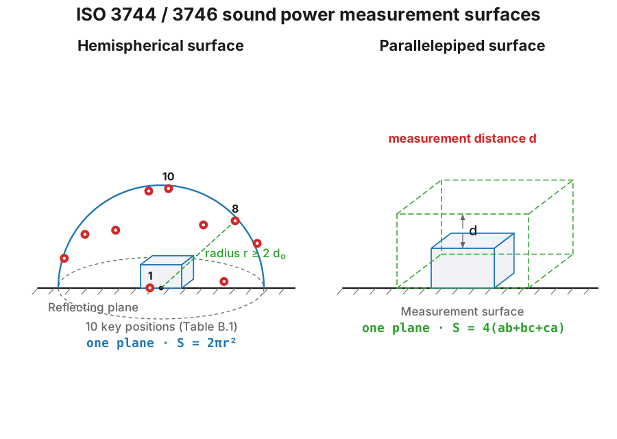
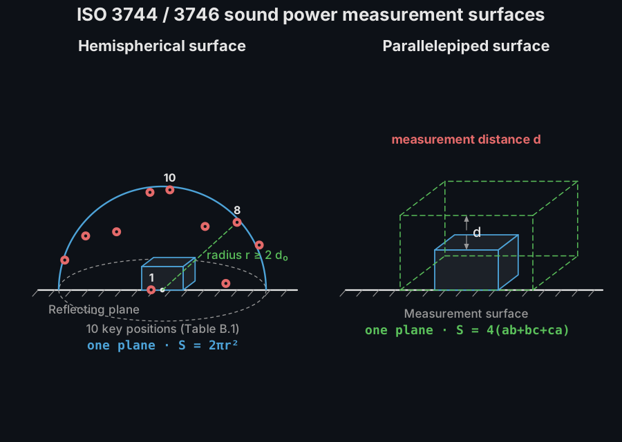
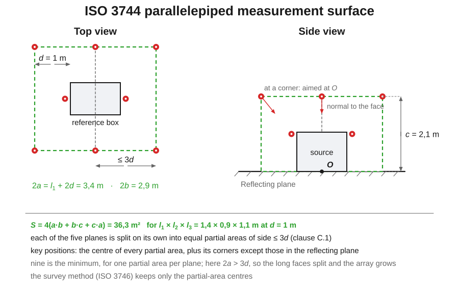
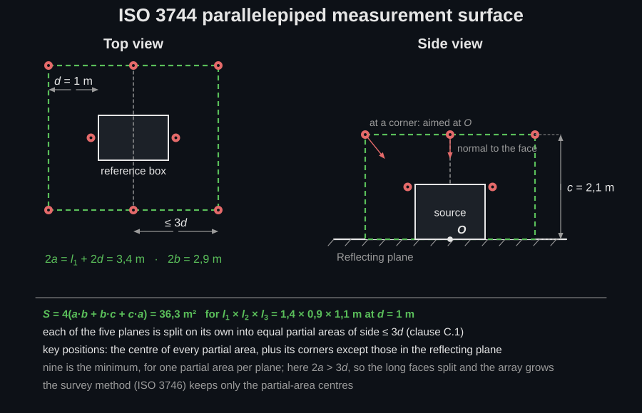
The box surface carries its own array, and it is not the Annex B hemisphere array: measurement_positions deliberately raises for a box, because ISO 3744 defines those positions by area subdivision instead (Annex C, normative). Each of the five planes of the measurement surface is considered on its own and divided into equal partial areas whose side does not exceed $3d$; the key positions are then the centre of every partial area plus its corners, excluding the corners that intrude into the reflecting plane, which gives a minimum of nine positions when one partial area covers each plane (clause C.1; ten for a triangular subdivision). The survey method keeps only the partial-area centres. The reference direction of each microphone is normal to its face, except at a corner of the surface, where it points at the origin $O$ of the reference box (clause 7.2.2).

levels_positions is not any array of decibels: it is the per-position, per-band time-averaged level with the source running in its declared operating mode, taken through a chain the standard specifies. The whole instrumentation system — microphones, cables and the windscreen if one is fitted — shall meet IEC 61672-1 class 1, and the filters IEC 61260 class 1 (clause 5.1). A class 1 IEC 60942 sound calibrator is applied to each microphone before and after each series to check the whole measuring chain, and, with no adjustment in between, the two readings shall differ by no more than 0,5 dB; beyond that the series is discarded, not corrected (clause 5.2). The system’s own compliance is verified in a traceable laboratory at intervals not exceeding two years, the calibrator’s at intervals not exceeding one year. The mechanics of that check are on Calibration.

Each microphone is oriented with its reference direction normal to the measurement surface, and at a corner of a box surface pointing at the origin $O$ (clause 7.2.2) — which is why a free-field capsule and a diffuse-field capsule are aimed differently on the same stand.

Each level is time-averaged over a typical period of operation: the interval should be 20 s or longer and shall be at least 10 s, and it has to be stated in the test report (clause 8.2.1). A traversing microphone integrates over an integer number of full traverses, and at least two. The background reading is taken immediately before or immediately after the source reading, at the same positions and over the same interval — so background_levels is a same-day, same-array (NM, NB) measurement, not a spectrum copied from another session, and pairing mismatched readings is the most common way a $K_1$ ends up wrong.

import numpy as np
from phonometry import emission

# Octave-band SPL (dB) at the 10 hemisphere positions of ISO 3744 (Annex B),
# with the source running, plus the background spectrum with it switched off.
freqs = np.array([63, 125, 250, 500, 1000, 2000, 4000, 8000])
base = np.array([70.0, 74.0, 78.0, 80.0, 79.0, 76.0, 72.0, 66.0])
rng = np.random.default_rng(0)
levels = base + rng.normal(0.0, 0.5, size=(10, 8))     # (positions, bands)
background = np.full((10, 8), 55.0)

# ISO 3744 Annex B microphone coordinates on a radius-1.5 m hemisphere.
mic_xyz = emission.measurement_positions("hemisphere", radius=1.5, reflecting_planes=1)
print(mic_xyz.shape)                                    # (10, 3)

res = emission.sound_power_pressure(
    levels, "hemisphere", radius=1.5, reflecting_planes=1,
    background_levels=background, frequencies=freqs,
    room=emission.RoomEnvironment(reverberation_time=0.6, volume=300.0),  # -> K2
)
print(round(res.surface_area, 2))                       # 14.14 m^2 (= 2*pi*1.5^2)
print(round(float(res.environmental_correction[0]), 2)) # K2 = 2.32 dB
print(round(res.sound_power_level_a, 1))                # LWA = 92.4 dB
print(round(res.uncertainty, 1))                        # U = 3.0 dB (2*sigma_R0)
print(np.round(res.sound_power_level, 1))               # per-band LW

res.plot()   # sound power level bars per band, LWA in the title (needs matplotlib)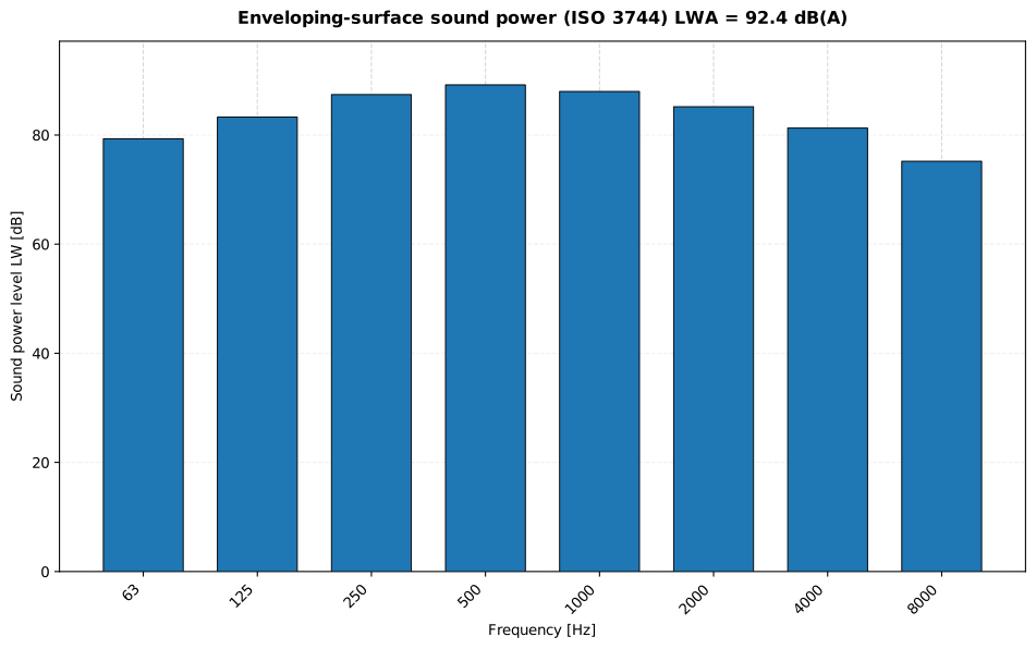

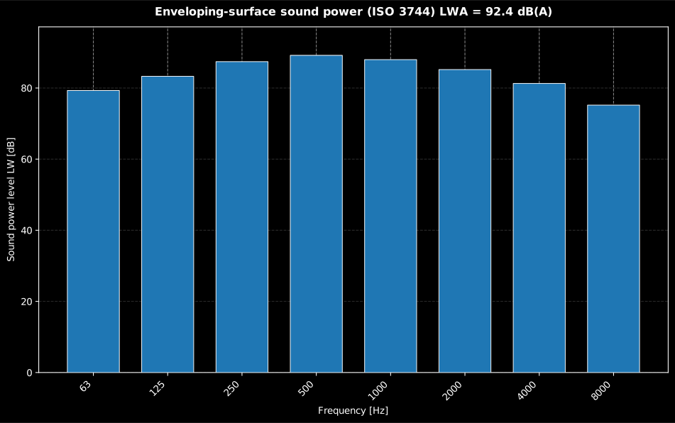
One bar per band: the energy-averaged surface pressure minus the background ($K_1$) and environmental ($K_2$) corrections plus the surface term $10{\log }_{10}(S/S_0)$ gives $L_W(f)$, and the A-weighted energy sum across bands gives the single-number $L_{W\mathrm{A}}$ in the title.

import matplotlib.pyplot as plt
import numpy as np
from phonometry import emission

# Octave-band SPL (dB) at the 10 hemisphere positions of ISO 3744 (Annex B),
# with the source running, plus the background spectrum with it switched off.
freqs = np.array([63, 125, 250, 500, 1000, 2000, 4000, 8000])
base = np.array([70.0, 74.0, 78.0, 80.0, 79.0, 76.0, 72.0, 66.0])
rng = np.random.default_rng(0)
levels = base + rng.normal(0.0, 0.5, size=(10, 8))     # (positions, bands)
background = np.full((10, 8), 55.0)
res = emission.sound_power_pressure(
    levels, "hemisphere", radius=1.5, reflecting_planes=1,
    background_levels=background, frequencies=freqs,
    room=emission.RoomEnvironment(reverberation_time=0.6, volume=300.0),  # -> K2
)

# res is the SoundPowerResult computed above. One line:
res.plot()
plt.show()

# By hand: a bar spectrum of LW with the A-weighted total in the title.
freqs = res.frequencies
positions = np.arange(freqs.size)
fig, ax = plt.subplots()
ax.bar(positions, res.sound_power_level, width=0.7, color="#1f77b4")
ax.set_xticks(positions)
ax.set_xticklabels([f"{f:g}" for f in freqs], rotation=45, ha="right")
ax.set_xlabel("Frequency [Hz]")
ax.set_ylabel("Sound power level LW [dB]")
ax.set_title(
    f"Enveloping-surface sound power (ISO 3744)  "
    f"LWA = {res.sound_power_level_a:.1f} dB(A)")
plt.show()

The A-weighted total $L_{W\mathrm{A}}$ is combined from the band powers with the ISO 3744 Annex E A-weighting corrections, so it needs frequencies. Passing a RoomEnvironment as room (reverberation_time + volume, or absorption_area, or mean_absorption_coefficient + room_surface) enables $K_2$; omit it and the field is treated as free ($K_2=0$). If the background margin drops below the grade criterion or $K_2$ exceeds the validity limit, a SoundPowerWarning flags that the levels are upper bounds; the determination still returns.

Both corrections subtract energy from the surface level, so overestimating either one understates the emission. That is why the standards cap them, and why most disputes over an enveloping-surface result trace back to one of these habits:

• $K_1$ has a cliff, not a slope. At a 15 dB margin the correction is a negligible 0.14 dB; at the 6 dB engineering criterion it is already 1.26 dB, the largest value the grade accepts. Below the criterion the standard does not let the formula run on: $K_1$ is capped and the result is reported as an upper bound. Never extrapolate the subtraction into a smaller margin; raise the margin (quieter site, closer surface) or switch to the intensity method.
• $K_1$ assumes a stationary background. The source-off reading must be taken at the same positions with the room in the same state, and the background energy must be the same during both readings. A ventilation system that cycles or a vehicle passing during either reading invalidates the pair; the energy subtraction also assumes source and background are incoherent, which holds for unrelated noise but not for the source’s own reflections.
• $K_2$ removes the average room build-up, not discrete reflections. A nearby wall, a trolley or another machine just outside the surface adds a specular contribution concentrated at a few microphones. That imbalance shows up in the apparent directivity index $D{I}_i^{\ast }$, and no room-average correction can remove it: move the surface, remove the reflector or treat it with absorption.
• $K_2$ is only as good as $A$. With $A$ from Sabine ($0.16V/T$), errors in the reverberation time or the volume propagate directly. At the $K_2=4\text{dB}$ validity limit about 60 % of the measured energy is room, not source, and a 20 % error in $A$ still moves $L_W$ by about 0.5 dB. Prefer a measured $T_{60}$ over a guessed absorption coefficient, and keep the measurement distance small enough that $K_2$ stays well under the limit.

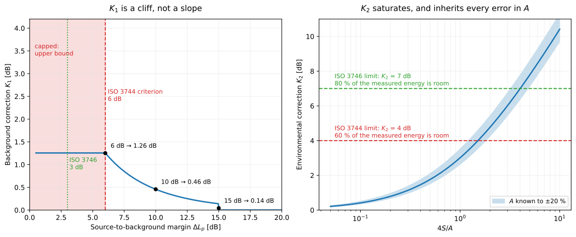
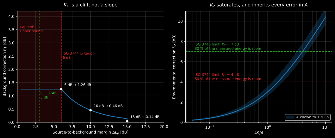
The two corrections have opposite shapes. $K_1$ is flat until the margin closes and then rises steeply, which is why the standards cap it at the criterion rather than let the formula run on; $K_2$ grows without bound as the surface fills the room, and the ±20 % band shows what an estimated $A$ costs at the validity limit.

import matplotlib.pyplot as plt
import numpy as np

# K1 is read out of sound_power_pressure itself, by sweeping the background
# under a fixed surface level; K2 is its own closed form.
margins = np.linspace(0.5, 20.0, 200)
k1 = [float(emission.sound_power_pressure(
          np.full((10, 1), 80.0), "hemisphere", radius=2.0,
          background_levels=np.full((10, 1), 80.0 - m),
          frequencies=np.array([1000.0])).background_correction[0])
      for m in margins]
ratio = np.geomspace(0.05, 10.0, 200)

fig, (axl, axr) = plt.subplots(1, 2, figsize=(12, 5))
axl.plot(margins, k1)
axl.axvline(6.0, linestyle="--")        # ISO 3744 criterion
axl.set(xlabel="ΔLp [dB]", ylabel="K1 [dB]", ylim=(0, 4.2))
axr.semilogx(ratio, 10.0 * np.log10(1.0 + ratio))
axr.axhline(4.0, linestyle="--")        # ISO 3744 validity limit
axr.set(xlabel="4S/A", ylabel="K2 [dB]")
plt.show()

One correction the enveloping-surface formula does not carry is meteorological. Eq. 18 assumes the reference characteristic impedance of air, so the determination is a determination “for the meteorological conditions at the time and place of the test” (clause 8.2.5). At altitudes above 500 m or temperatures below 10 °C that becomes a bias, and clause 8.2.5 then requires the result to be carried to reference conditions per Annex G, which is normative — the same kind of term the ISO 3741 and ISO 3745 sections write out explicitly as $C_1$ and $C_2$. The size of it: clause H.4.2.7 states that below 500 m no meteorological or radiation-impedance correction is required, that at 120 m and 23 °C the correction is zero, and that at 500 m it reaches 0.6 dB. Two of those three hold. Annex G, which is the normative text that same clause points at, puts the correction at 0.394 dB at 500 m and 23.0 °C, and the zero at 120 m comes out exact, which is what shows its equations are being read as the standard intends. The 0.6 dB is a misprint, and it is recorded with the arithmetic in the errata registry. sound_power_pressure implements no such term and takes no temperature or pressure argument at all, so a determination at a mountain plant or outdoors in winter adds the Annex G correction afterwards: reference_atmosphere_correction evaluates $C_1+C_2$ from the temperature and the static pressure (or the altitude, through Eq. G.2), and section 4 shows it applied, since Eq. G.1 adds it to $L_W$ exactly as Eq. G.3 adds it to $L_J$.

Returns a SoundPowerResult: sound_power_level (per-band $L_W$), surface_pressure_level ($L_p$ after $K_1$/$K_2$), mean_pressure_level, background_correction/environmental_correction ($K_1$/$K_2$), directivity_index (apparent $D{I}_i^{\ast }$ per microphone position and frequency band, shape (NM, NB); ISO 3744 clause 8.4), surface_area, sound_power_level_a ($L_{W\mathrm{A}}$), uncertainty (expanded, 95 %) and grade. measurement_positions('hemisphere', radius=…, reflecting_planes=…, tones=…, grade=…) returns the normative (N, 3) microphone coordinates (Table B.1 for tonal sources, B.2 for broadband). Those coordinates plot directly with plot_microphone_positions, which draws the array on its measurement surface in 3-D, numbered as in the standard.

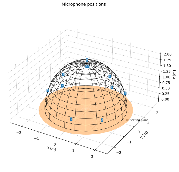
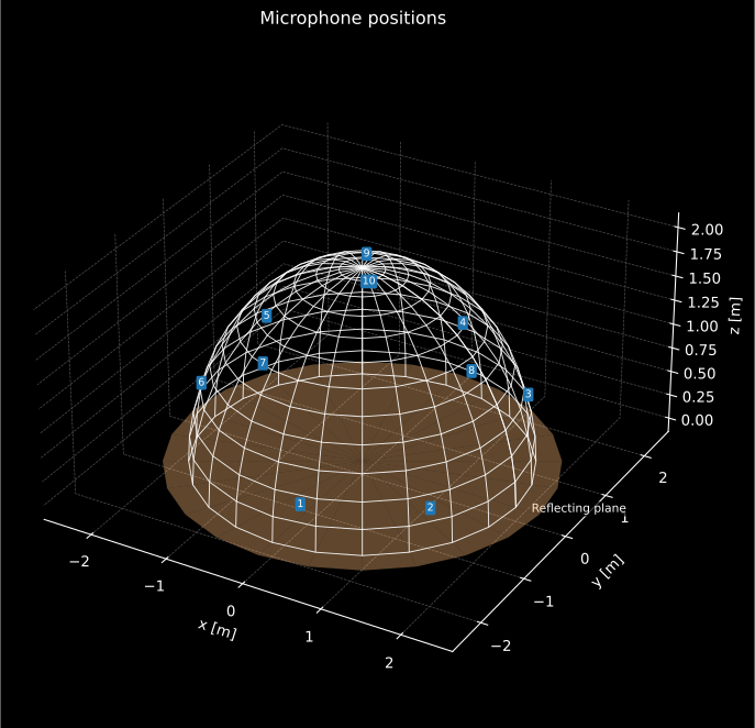
Where the ten Annex B microphones actually sit on the 2 m hemisphere: the heights are staggered so the array samples the whole surface evenly, which is what lets the plain energy average of the ten levels stand in for the surface integral.

import matplotlib.pyplot as plt
from phonometry import emission

# The 10 ISO 3744 Annex B microphones on a 2 m hemisphere.
emission.plot_microphone_positions(emission.measurement_positions("hemisphere", radius=2.0),
                                   radius=2.0)
plt.show()

Ten is the count for one reflecting plane. Against two planes the array is the five key positions 2, 3, 6, 7 and 9 of Table B.2; in a corner, against three planes, it is the three positions 1, 2 and 3 of Table B.3 (clause 8.1.1). The survey method uses coarser arrays again — four positions over one plane.

Those counts are a starting point, not a result. Clause 8.1.1 requires additional positions if any one of three conditions holds:

• a) the range of the A-weighted levels across the key positions exceeds 10 dB over one reflecting plane, 5 dB over two, or 3 dB over three;
• b) the apparent A-weighted directivity index exceeds 5 dB in any direction;
• c) a large source radiates from only a small part of itself — the openings of an otherwise enclosed machine being the standard’s own example.

The two have different answers. Condition a) is met by adding positions 11 to 20 of the same table (or, equivalently, by repeating the key array with the source rotated −60° for Table B.1 or 180° for Table B.2): the surface is still sampled evenly, so the plain energy average still applies. Conditions b) and c) are met by a localized investigation — extra positions concentrated around the maximum, numerically equal to the level range found — and those positions carry unequal segment areas, so the mean must then be the area-weighted one of clause 8.2.2.2 and not the equal-area average sound_power_pressure computes. Note 3 adds a priority rule that saves a lot of wasted work: when the background at any position is within 6 dB of the highest source level, reduce the background before adding positions, because a background that close is what is moving $D{I}_i^{\ast }$ in the first place.

Both gates are one line each on the result the page has already computed:

import numpy as np

# The band-summed level per position (A-weight the bands first for the
# standard's own A-weighted range; here the source is broadband enough that it
# makes no difference to the verdict).
lp_a = 10.0 * np.log10(np.sum(10.0 ** (0.1 * levels), axis=1))
print(round(float(lp_a.max() - lp_a.min()), 2))       # 0.76 dB: condition a) clear
print(round(float(np.abs(res.directivity_index).max()), 2))   # 1.1 dB: b) clear

$D{I}_i^{\ast }$ is the apparent directivity index of clause 8.4, the excess of the background-corrected level at position $i$ over the surface average, per position and per band; it is what the $K_2$ pitfall above meant by “shows up in the apparent directivity index”. A machine that radiates 5 dB more towards one microphone than the surface average does not have a broken array — it has a directivity the ten positions cannot resolve.

When the highest accuracy is required, ISO 3745 measures sound power in a qualified anechoic or hemi-anechoic room, where the free field lets a fixed array of microphones sample the radiated sound pressure directly. It is the grade-1 counterpart to the enveloping-surface method of Section 1, with standardized microphone coordinates, a per-position background correction and an explicit meteorological correction.

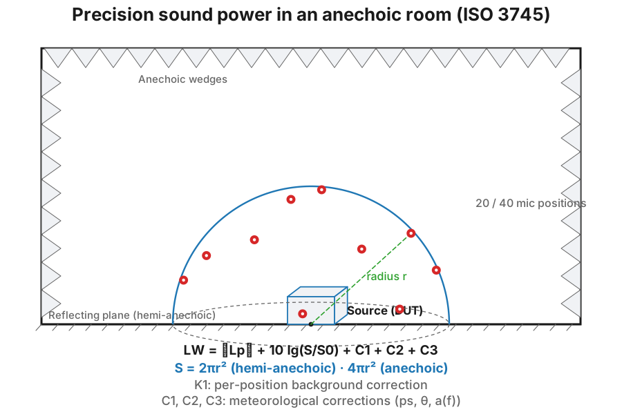
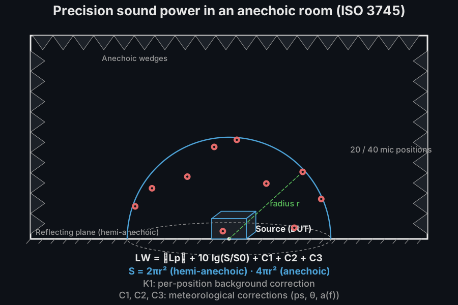
The left-hand panel of the clip below is what that room is for. With the boundaries absorbing, a microphone sees only what the source sends its way, so the level falls with distance and the array has to sample a whole surface — which is why the only geometry the method needs, once the room is qualified, is the surface term $10{\log }_{10}(S/S_0)$. The right-hand panel is the reverberation-room alternative of ISO 3741, and both end on the same $L_W$.

Sound power level (Clause 8). The band sound power level is the surface-averaged pressure level plus the surface term and the corrections:

with $S=4\pi r^2$ over the sphere or $S=2\pi r^2$ over the hemisphere, $S_0=1{\text{m}}^2$. $C_1$ and $C_2$ are the meteorological corrections (reference and radiation-impedance terms); $C_3$ accounts for air absorption over the measurement radius. The microphone positions are the standardized unit-vector arrays of Tables D.1 (sphere), E.1 (hemisphere) and E.2 (hemisphere, broadband).

There is no separate $K_1$ term in that formula because $\overline{L_p}$ — unprimed, unlike section 1’s — is the surface average of the levels after each one has been background-corrected on its own,

(clause 9.4.3.1). So the correction lives inside the average, one $K_{1i}$ per position, rather than being subtracted from the mean the way ISO 3744 does it. mean_pressure_level is the raw energy average and surface_pressure_level the corrected one, which is the $\overline{L_p}$ of the formula above.

The radius is not free (clauses 8.1/8.2). It must satisfy $r\ge 2d_0$ with $d_0$ the distance from the acoustic centre to the furthest point of the source (in a hemi-anechoic room, $r\ge 2d_0$ or $r\ge 3h_0$, whichever is larger, $h_0$ being the height of the acoustic centre above the floor), $r\ge \lambda /4$ at the lowest frequency of interest, and $r\ge 1$ m — 0.5 m only for a small, low-noise source over a limited band — with the whole surface inside the region qualified per Annex A or B. Worked: a 0.6 × 0.5 × 0.7 m benchtop source has $d_0=\sqrt{0.3^2+0.25^2+0.7^2}=0.80$ m, so $r\ge 1.6$ m; at a lowest band of 100 Hz, $\lambda /4=0.86$ m does not bind and neither does the 1 m floor. The radius=1.0 of the examples below therefore fits only a source under about 0.5 m of characteristic dimension.

The array is not free either. Positions 1 to 20 are used first, and 21 to 40 are added only when the difference between the highest and lowest level in any band of interest is not less than half the number of positions — a check on data the reader already has, levels.max(0) - levels.min(0) >= 0.5 * levels.shape[0]. If 40 positions still fail it, a localized investigation is required and the positions then carry unequal areas, which is what areas= is for.

import numpy as np
from phonometry import emission

# The 40 standardized hemisphere positions (unit vectors scaled by the radius).
pos = emission.precision_positions("hemisphere", radius=1.0, count=40)
print(pos.shape)                      # (40, 3)

# Octave/third-octave band SPL (dB) at each of the 40 positions; here a uniform
# 74 dB in one band. The result carries S = 2*pi*r^2 and LW with C1+C2+C3.
levels = np.full((40, 1), 74.0)
res = emission.sound_power_anechoic(levels, "hemisphere", radius=1.0)
print(round(res.surface_area, 3))                 # 6.283  (2*pi*1^2)
print(np.round(res.sound_power_level, 2))         # [81.85]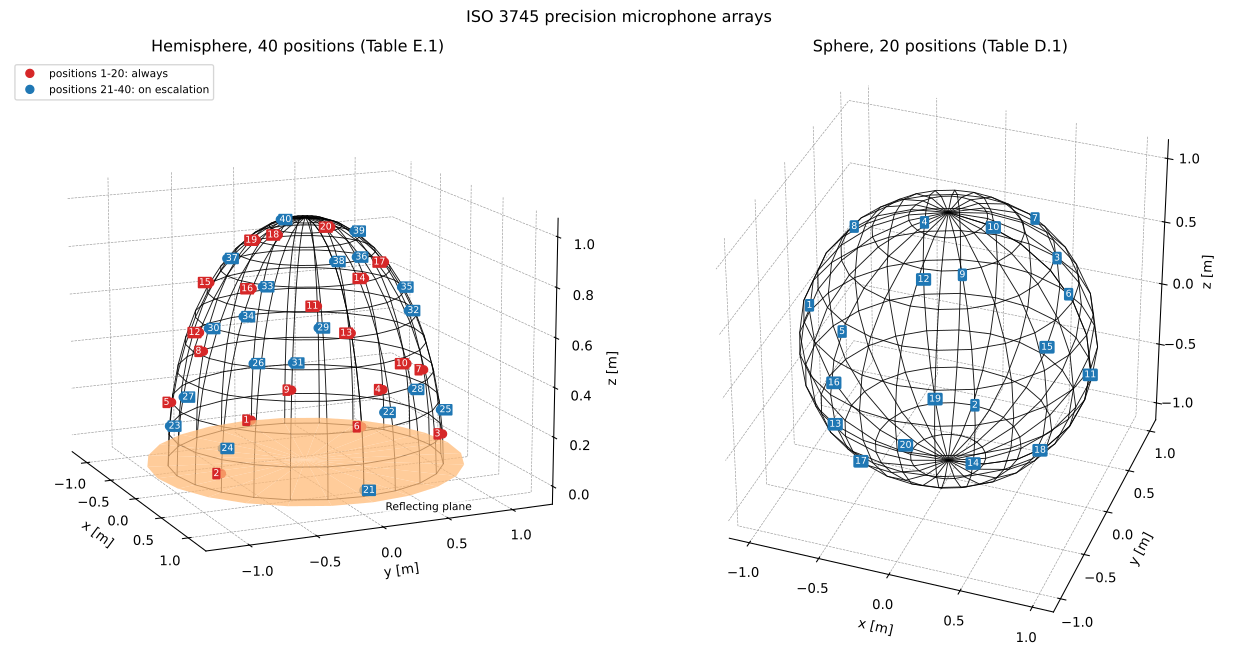

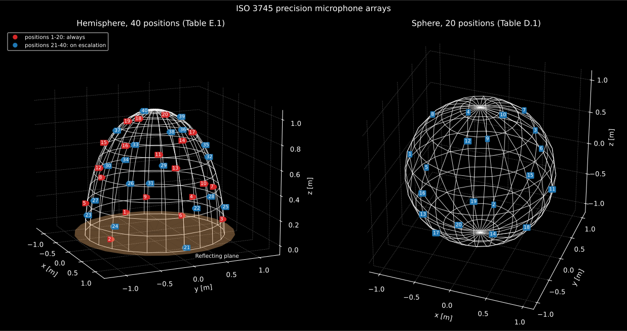
The precision arrays, drawn from the same precision_positions call the snippet above makes. The first twenty sample the surface on their own; the second twenty are added only when the band level range triggers the escalation, and a localized investigation after that carries unequal areas.

import matplotlib.pyplot as plt

fig, (axl, axr) = plt.subplots(1, 2, subplot_kw={"projection": "3d"})
emission.plot_microphone_positions(
    emission.precision_positions("hemisphere", radius=1.0, count=40),
    ax=axl, radius=1.0)
emission.plot_microphone_positions(
    emission.precision_positions("sphere", radius=1.0, count=20),
    ax=axr, radius=1.0)
plt.show()

Background and meteorological corrections. The $K_1$ background correction is applied per position and floored where the signal-to-background difference is small (Eq. 11); the meteorological correction is evaluated from the measured temperature and static pressure.

import numpy as np
from phonometry import emission

# K1 for a 6 dB signal-to-background difference in a <=200 Hz edge band: the
# floor is 1.26 dB (Eq. 11). Source and background levels are [positions, bands].
k1 = emission.precision_background_correction(
    np.array([[56.0]]), np.array([[50.0]]), np.array([200.0]))
print(round(float(k1[0, 0]), 4))      # 1.2563

# Meteorological corrections at the 23 C, 101.325 kPa reference (Eq. 16):
mc = emission.meteorological_corrections(23.0, 101.325)
print(round(mc.c1, 4), round(mc.c2, 4))   # -0.1282 0.0

# Expanded uncertainty (Clause 10.5 EXAMPLE): sigma_R0 = 0.5, sigma_omc = 2.0,
# k = 2 -> U = 4.1 dB.
print(round(emission.precision_uncertainty(0.5, 2.0, 2.0), 3))   # 4.123

The MeteorologicalCorrection is a pair of scalars (plus the per-band $C_3$ when the attenuation coefficient is supplied per band) rather than a plottable spectrum: the corrections fold into the PrecisionSoundPowerResult as its c1/c2/c3 fields, and the .report() fiche prints them on its measurement-basis strip.

The margins and the intervals behind those numbers are stricter than section 1’s. The background, averaged over all positions, shall be at least 6 dB below the source level in every band and at least 10 dB below from 250 Hz to 5 kHz (clause 5.2.1.1) — a band that cannot reach it may instead be excluded from the range of interest if its corrected A-weighted band power is at least 15 dB below the highest (clause 5.2.1.2). Where the margin falls short anyway, clause 9.4.2 freezes $K_{1i}$ at the value the criterion produces, 1.26 dB for the bands at and below 200 Hz and at and above 6,3 kHz, 0,46 dB from 250 Hz to 5 kHz — and then requires the test report, and the tables and graphs in it, to state that those bands are upper bounds. precision_background_correction applies exactly that rule; declaring the omission is the reader’s job.

The averaging is longer than ISO 3744’s: at least 30 s in the bands centred at and below 160 Hz and at least 10 s from 200 Hz up (clause 9.4.1), with the interval stated in the report, and at least two full traverses when a traversing microphone is used. The background is measured immediately before or immediately after the source, at the same positions and over the same interval. Forty positions at 30 s in the low bands is why a grade-1 run takes so much longer than the grade-2 one of section 1 — the cost of the grade is mostly time.

The last two are the whole uncertainty story, and the default hides it: left alone, sigma_omc = 0 claims a perfectly repeatable installation and the fiche prints $U=1.0$ dB. The 4.1 dB the example below reports is what the same determination costs once the clause 10.5 EXAMPLE value ${\sigma }_{\text{omc}}=2.0$ dB is admitted.

Over several bands sound_power_anechoic returns a plottable PrecisionSoundPowerResult carrying the per-band $L_W$ and the A-weighted total:

import numpy as np
from phonometry import emission

# A mid-frequency-peaked machine measured over the 40-position hemisphere array
# (Annex E). levels_positions is the (40, NB) surface pressure spectrum: a base
# spectrum peaked near 1 kHz plus a small per-position spatial spread.
freqs = np.array([125, 250, 500, 1000, 2000, 4000, 8000], float)
base = 70.0 + 8.0 * np.exp(-(np.log2(freqs / 1000.0) ** 2) / 2.0)
rng = np.random.default_rng(7)
levels = base[None, :] + rng.normal(0.0, 1.0, (40, freqs.size))

# sigma_omc is the operating-and-mounting standard deviation of Clause 10.5;
# with the EXAMPLE value 2.0 dB and the default coverage factor k = 2 the
# expanded uncertainty U = k*sqrt(sigma_R0^2 + sigma_omc^2) is the 4.1 dB the
# fiche below prints. Left at its default of 0 it reports 1.0 dB.
result = emission.sound_power_anechoic(levels, "hemisphere", radius=1.0,
                                       frequencies=freqs, sigma_omc=2.0)
print(round(result.sound_power_level_a, 1))   # 89.3
print(round(float(result.uncertainty), 1))    # 4.1  dB
result.plot()   # LW spectrum, LWA in the title (needs matplotlib)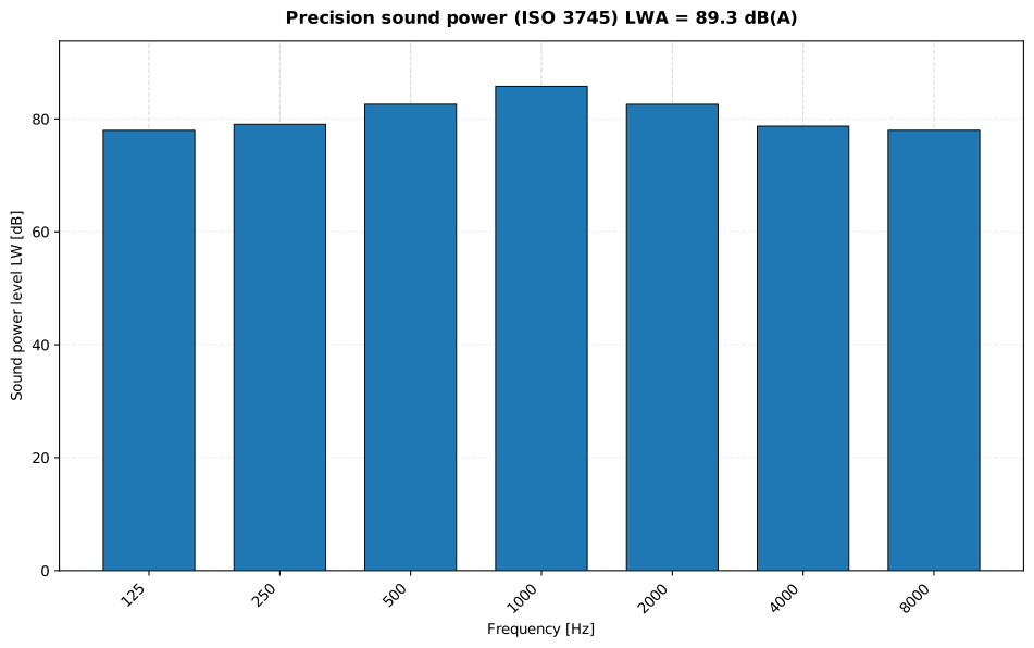

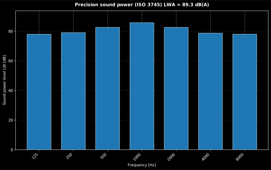
One bar per band: the surface-averaged pressure plus the area, background and meteorological corrections give $L_W(f)$, and the A-weighted energy sum across bands gives the single-number $L_{W\mathrm{A}}$ in the title.

import matplotlib.pyplot as plt
import numpy as np
from phonometry import emission

# A mid-frequency-peaked machine measured over the 40-position hemisphere array
# (Annex E). levels_positions is the (40, NB) surface pressure spectrum: a base
# spectrum peaked near 1 kHz plus a small per-position spatial spread.
freqs = np.array([125, 250, 500, 1000, 2000, 4000, 8000], float)
base = 70.0 + 8.0 * np.exp(-(np.log2(freqs / 1000.0) ** 2) / 2.0)
rng = np.random.default_rng(7)
levels = base[None, :] + rng.normal(0.0, 1.0, (40, freqs.size))
result = emission.sound_power_anechoic(levels, "hemisphere", radius=1.0, frequencies=freqs)

# result is the PrecisionSoundPowerResult computed above. One line:
result.plot()
plt.show()

# By hand: a bar spectrum of LW with the A-weighted total in the title.
freqs = result.frequencies
positions = np.arange(freqs.size)
fig, ax = plt.subplots()
ax.bar(positions, result.sound_power_level, width=0.7, color="#1f77b4")
ax.set_xticks(positions)
ax.set_xticklabels([f"{f:g}" for f in freqs], rotation=45, ha="right")
ax.set_xlabel("Frequency [Hz]")
ax.set_ylabel("Sound power level LW [dB]")
ax.set_title(
    f"Precision sound power (ISO 3745)  LWA = {result.sound_power_level_a:.1f} dB(A)")
plt.show()

A sound power determination ends as a document. Every result of this page stays plottable while it is being worked on (res.plot() draws the same $L_W$ spectrum interactively that the fiche typesets), and the report step wraps it into the deliverable. Both the enveloping-surface result (SoundPowerResult, ISO 3744/3746) and the precision result (PrecisionSoundPowerResult, ISO 3745) expose a .report() method that writes a one-page PDF fiche laid out like a sound-power test sheet: the standard-basis line naming the applied method and accuracy grade, an optional metadata header (client, noise source, test environment, instrumentation, climate, date), a per-band table (nominal octave/one-third-octave frequency, the surface sound-pressure level $L_p$ and the band sound-power level $L_W$), the sound-power spectrum $L_W(f)$ with a nominal band axis, and a boxed A-weighted sound power level $L_{W\mathrm{A}}$ (dB re 1 pW) with the total $L_W$, the expanded uncertainty $U$ and the measurement surface area $S$ alongside.

The metadata is supplied through a ReportMetadata, whose applicable fields here are the source description (specimen), the test environment (test_room), the client, the instrumentation, the temperature, relative humidity and ambient pressure, the date of test (test_date) and the footer identity (laboratory, operator, report_id, notes); the measurement surface area $S$ comes from the result itself and is printed in the result box and the basis strip, together with the applied corrections (the background $K_1$ and environmental $K_2$ for the ISO 3744/3746 surface method, or the meteorological $C_1$/$C_2$/$C_3$ for the ISO 3745 precision method). Supplying requirement adds a PASS/FAIL verdict against a declared A-weighted sound-power limit (a sound-power emission is a quantity where less is better, so the source passes at or below the limit). verbose=True adds the energy-averaged level $L_p^{\prime }$ to the table, and for the ISO 3744/3746 surface result it also adds the $K_1$/$K_2$ correction columns (the precision result has no $K_2$ at all and folds its per-position $K_1$ into the surface average, so the fiche prints $C_1$/$C_2$/$C_3$ on its basis strip in place of those columns). language="es" renders the Spanish fiche with comma decimals.

import numpy as np
from phonometry import ReportMetadata, emission

freqs = np.array([63, 125, 250, 500, 1000, 2000, 4000, 8000], float)
# Ten identical position spectra over a hemisphere of radius 4 m; background a
# uniform 10 dB below and an equivalent absorption area A = 1500 m^2 (so K1, K2
# are meaningful and within the engineering validity limit).
surface = np.array([72.0, 76, 80, 82, 81, 78, 73, 66])
res = emission.sound_power_pressure(
    np.tile(surface, (10, 1)), "hemisphere", radius=4.0,
    background_levels=np.tile(surface - 10.0, (10, 1)),
    frequencies=freqs, grade="engineering",
    room=emission.RoomEnvironment(absorption_area=1500.0),
)

res.report(
    "sound_power.pdf",
    metadata=ReportMetadata(
        client="Example manufacturing plant",
        specimen="Hydraulic power pack (floor-standing)",
        test_room="Hemi-anechoic room over a reflecting floor",
        instrumentation="Class 1 sound level meter (IEC 61672-1), s/n 0042",
        laboratory="Phonometry reference example",
        report_id="EXAMPLE-3744",
        requirement=105.0,
    ),
)   # LWA = 103.7 dB(A) re 1 pW -> declared limit 105 dB(A): PASS

The example fiche is regenerated with make reports and kept rendered in the repository; click the preview to open the PDF.

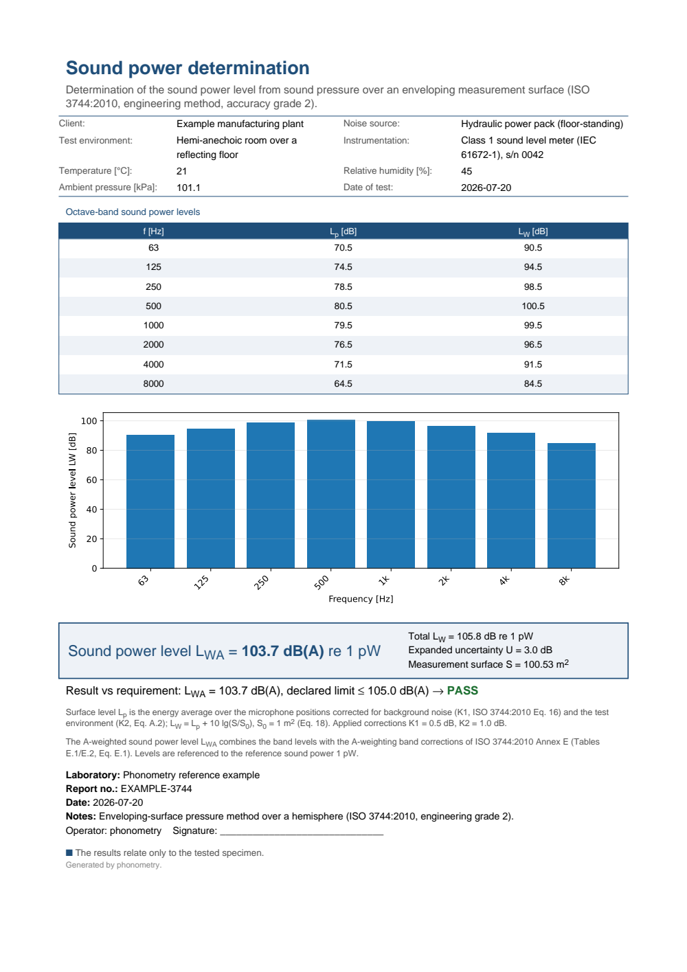
One-page ISO 3744 sound-power determination fiche: a header with the client, the noise source, the hemi-anechoic test environment and the instrumentation and climate, the octave-band table (63 Hz to 8 kHz) of surface sound-pressure levels Lp and band sound-power levels LW, the sound-power spectrum LW(f) with a nominal band axis, the boxed A-weighted sound power level LWA = 103.7 dB(A) re 1 pW with the total LW = 105.8 dB, the expanded uncertainty U = 3.0 dB and the measurement surface S = 100.53 m2, and a PASS verdict against the declared 105 dB(A) limit, closed by a basis strip stating the applied K1 = 0.5 dB and K2 = 1.0 dB corrections.

Download the report (PDF)

The precision result writes the same sheet from the ISO 3745 side, with the meteorological corrections on its basis strip in place of the $K_1$/$K_2$ pair. This is the 40-position hemisphere measurement of section 2, the one whose spectrum is plotted above:

from phonometry import ReportMetadata

result.report(
    "precision-sound-power.pdf",
    metadata=ReportMetadata(
        client="Example manufacturing plant",
        specimen="Mid-frequency-peaked machine",
        test_room="Qualified anechoic room, 40-position hemisphere array",
        measurement_standard="ISO 3745",
    ),
)   # LWA = 89.3 dB(A) re 1 pW, U = 4.1 dB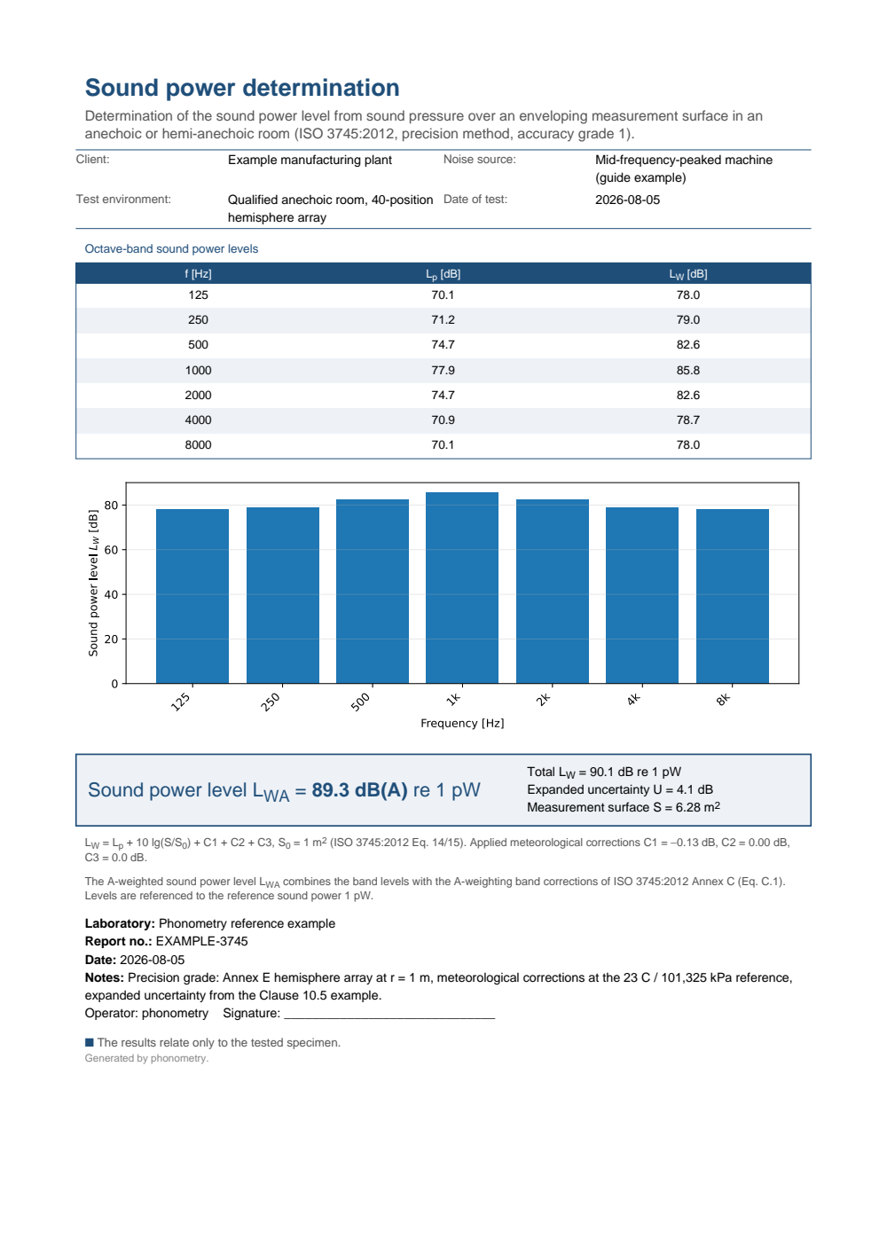

One-page ISO 3745 precision sound-power fiche: a header with the client, the noise source and the qualified anechoic room with its 40-position hemisphere array, the octave-band table from 125 Hz to 8 kHz of surface sound-pressure levels Lp and band sound-power levels LW (78.0, 79.0, 82.6, 85.8, 82.6, 78.7 and 78.0 dB), the LW spectrum peaking at 1 kHz, and the boxed A-weighted sound power level LWA = 89.3 dB(A) re 1 pW with the total LW = 90.1 dB, the expanded uncertainty U = 4.1 dB and the measurement surface S = 6.28 m2, over a basis strip stating the applied meteorological corrections C1 = -0.13 dB, C2 = 0.00 dB and C3 = 0.0 dB.

Download the report (PDF)

Everything above describes a source that runs steadily for the whole averaging interval: Eq. 18 reports a rate of energy flow, and it characterises the machine only while the machine is time-invariant. A press stroke, a door slam or a pneumatic exhaust radiates its energy in a fraction of a second and then stops, so the standard gives it a quantity of its own, the sound energy level

(clauses 3.22 and 3.23): the energy the event radiates, in decibels re 1 pJ, in place of the power it does not have. Its determination (clause 8.3, and clause 8.4 of ISO 3746 for the survey grade) is the chain of section 1 with one substitution. Each microphone records the single event time-integrated sound pressure level

(clause 3.4) through a window that encompasses the whole burst, at every position at once (a traversing microphone is not permitted, clause 8.3.1), and $L_E$ then goes wherever $L_p$ went: the energy average over the positions of 8.2.2 (clause 8.3.3), the background correction $K_1$ (Eq. 21) and the environmental correction $K_2$ (Eq. 22), the surface term (Eq. 23):

The two quantities meet on a steady source. Over a window of duration $T$ the integral of a constant $p^2$ is $T{p}^2$, so $L_E=L_{p,T}+10{\log }_{10}(T/T_0)$ with $T_0=1$ s (clause 3.4 NOTE 1), and the energy a steady source radiates in $T$ seconds is $L_J=L_W+10{\log }_{10}(T/T_0)$: a machine of 90 dB running for 10 s has put out $L_J=100$ dB. That identity is what the figure below draws, and what the library’s own tests pin the sound energy chain to, field by field.

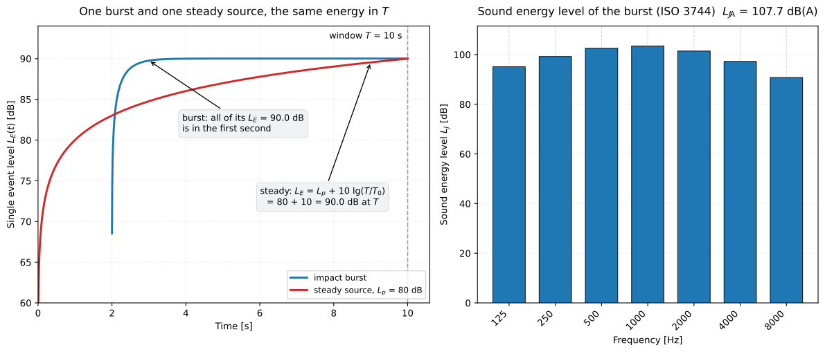
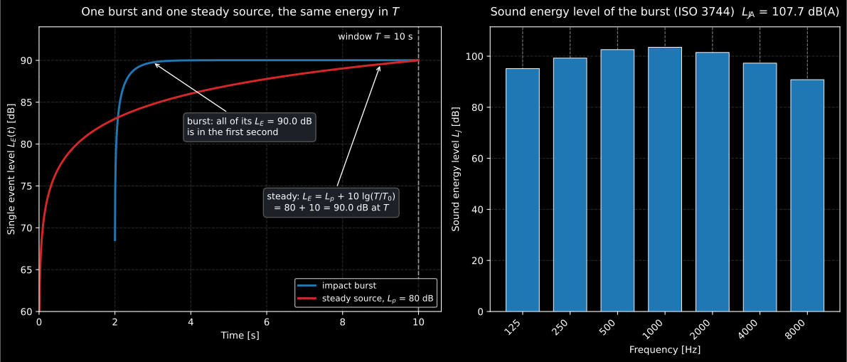
Left, the running single event level of an impact burst and of a steady 80 dB source through a 10 s window: the burst’s 90 dB is all there within a second of the impact, the steady source climbs as $10{\log }_{10}(t/T_0)$ and reaches the same 90 dB at $T$. Right, the octave-band $L_J$ of the same press stroke measured over a 2 m hemisphere, with the A-weighted total in the title.

import numpy as np
from phonometry import emission

# A press stroke measured at the 10 hemisphere positions of ISO 3744 (r = 2 m),
# five strokes one at a time: (events, positions, bands), octaves 125 Hz - 8 kHz.
bands = np.array([125, 250, 500, 1000, 2000, 4000, 8000], dtype=float)
stroke = np.array([84.0, 88.0, 91.0, 92.0, 90.0, 86.0, 80.0])   # single event levels, dB
rng = np.random.default_rng(83)
events = stroke + rng.normal(0.0, 0.8, size=(5, 10, bands.size))

burst = emission.sound_energy_pressure(
    events, "hemisphere", radius=2.0,
    background_levels=np.full((10, bands.size), 62.0),   # time-averaged over the same 10 s
    integration_time=10.0, frequencies=bands,
    room=emission.RoomEnvironment(reverberation_time=1.2, volume=900.0),   # -> K2
)
print(burst.events)                                        # 5 (Eq. 19 over the first axis)
print(round(float(burst.environmental_correction[0]), 2))  # K2 = 2.64 dB
print(np.round(burst.sound_energy_level, 1))               # per-band LJ, peaking at 103.5 dB at 1 kHz
print(round(burst.sound_energy_level_a, 1))                # LJA = 107.7 dB(A)

burst.plot()   # LJ per band, LJA in the title (needs matplotlib)

import matplotlib.pyplot as plt

# Left: the running single event level of the two sources. The burst decays
# with a 0.35 s time constant and holds an exposure of 90 dB; the steady
# source is 80 dB, so it reaches the same 90 dB at T = 10 s.
p0_sq = (20e-6) ** 2
e0 = p0_sq * 1.0
t = np.linspace(0.0, 10.0, 4001)
dt = t[1] - t[0]
burst_p2 = np.where(t >= 2.0, (e0 * 1e9 / 0.35) * np.exp(-(t - 2.0) / 0.35), 0.0)
steady_p2 = np.full_like(t, p0_sq * 1e8)
fig, (axl, axr) = plt.subplots(1, 2, figsize=(12.5, 5.4))
with np.errstate(divide="ignore"):
    axl.plot(t, 10 * np.log10(np.cumsum(burst_p2) * dt / e0), label="impact burst")
    axl.plot(t, 10 * np.log10(np.cumsum(steady_p2) * dt / e0), label="steady, 80 dB")
axl.set(xlabel="Time [s]", ylabel="Single event level LE(t) [dB]", ylim=(60, 94))
axl.legend()

# Right: the LJ spectrum is the result computed above.
burst.plot(ax=axr)
plt.show()

The standard asks for at least five events (clause 8.3.1), measured either one at a time or as one reading that spans them all, and reduces both to the level of one event at each position: the energy average of the $N_{\mathrm{e}}$ single readings,

or the one reading less the $10{\log }_{10}{N}_{\mathrm{e}}$ of the events it holds,

sound_energy_pressure takes the three forms levels_positions comes in: a (Ne, NM, NB) array of the events measured one at a time (Eq. 19, as in the snippet above), an (NM, NB) reading of one measurement encompassing events=Ne events (Eq. 20), or the (NM, NB) mean single event level already formed. Fewer than five events are accepted with a SoundPowerWarning, and mean_single_event_level exposes the same reduction on its own:

five_at_once = emission.mean_single_event_level(np.full((10, 1), 97.0), events=5)
print(round(float(five_at_once[0, 0]), 2))          # 90.01 dB: 97 - 10 lg 5 (Eq. 20)
one_by_one = emission.mean_single_event_level(np.array([89.0, 91.0, 90.0, 90.5, 89.5]))
print(round(float(one_by_one), 2))               # 90.06 dB: the energy mean (Eq. 19)

Clause 8.3.1 has the background measured as a time-averaged level over the same integration time $T$ as the events, and Eq. 21 forms $K_1$ from $\Delta L_E=\overline{L_E^{\prime }}-\overline{L_{p(\mathrm{B})}}$. Those two levels do not share a reference: $L_E$ is an energy re $E_0=p_0^2\cdot 1$ s and $L_p$ a mean-square pressure re $p_0^2$, and $K_1$ subtracts one energy from another. The energy the background contributes to a window of $T$ seconds is its own exposure over that window, $L_{p(\mathrm{B})}+10{\log }_{10}(T/T_0)$ (the same NOTE 1 identity), so that is what sound_energy_pressure compares the event level with, and why integration_time is required whenever background_levels is given. Read literally, a 62 dB background under a 78 dB burst in a 10 s window would look 16 dB down and earn no correction; as an energy it is 72 dB, the margin is the 6 dB engineering criterion, and $K_1$ is its full 1.26 dB. The errata registry records the reading. With the background in place, the criteria and the clamp are section 1’s: 6 dB to 15 dB for the engineering grade, 3 dB to 10 dB for the survey grade of ISO 3746, and a SoundPowerWarning when a band falls below them.

# 62 dB time-averaged over 10 s is 72 dB re E0; a 78 dB burst is then 6 dB above it.
k1 = emission.sound_energy_pressure(
    np.full((10, 1), 78.0), "hemisphere", radius=2.0,
    background_levels=np.full(1, 62.0), integration_time=10.0,
).background_correction
print(round(float(k1[0]), 2))    # K1 = 1.26 dB, the value at the 6 dB criterion

The identity with section 1 then holds to the last digit. The same ten positions, background and room, with every level raised by $10{\log }_{10}(T/T_0)$ for a 10 s window, give $L_J$ exactly 10 dB above $L_W$ in every band, and the same $K_1$, $K_2$ and expanded uncertainty, which clause 9.1 (Eq. 24) makes common to both quantities:

# The section 1 measurement read as a 10 s window: LJ = LW + 10 lg(T/T0) exactly.
octaves_hz = np.array([63, 125, 250, 500, 1000, 2000, 4000, 8000])
rng = np.random.default_rng(0)
ten_positions = np.array([70.0, 74.0, 78.0, 80.0, 79.0, 76.0, 72.0, 66.0]) + rng.normal(0.0, 0.5, size=(10, 8))
quiet = np.full((10, 8), 55.0)
workshop = emission.RoomEnvironment(reverberation_time=0.6, volume=300.0)
steady = emission.sound_power_pressure(
    ten_positions, "hemisphere", radius=1.5, reflecting_planes=1,
    background_levels=quiet, frequencies=octaves_hz, room=workshop,
)
ten_seconds = emission.sound_energy_pressure(
    ten_positions + 10.0, "hemisphere", radius=1.5, reflecting_planes=1,
    background_levels=quiet, integration_time=10.0, frequencies=octaves_hz, room=workshop,
)
print(np.round(ten_seconds.sound_energy_level - steady.sound_power_level, 6))   # 10.0 in every band
print(round(ten_seconds.sound_energy_level_a - steady.sound_power_level_a, 6))  # 10.0

Eq. 23 holds for the meteorological conditions of the test, and above 500 m of altitude or below 10 °C clause 8.3.6 requires the level to be carried to the reference 101.325 kPa and 23.0 °C by Annex G, $L_{J\mathrm{ref},\mathrm{atm}}=L_J+C_1+C_2$ (Eq. G.3), with

${\theta }_0=314$ K and ${\theta }_1=296$ K. $C_1$ is the reference-quantity correction through the characteristic impedance of the air (omitted when $K_2$ came from the absolute comparison test of A.2), $C_2$ the radiation-impedance correction of a monopole. Where the static pressure was not measured, Eq. G.2 estimates it from the altitude, $p_{\mathrm{s}}=p_{\mathrm{s},0}(1-a{H}_{\mathrm{a}}{)}^b$. Annex H.4.2.7’s check that the correction vanishes at 120 m and 23 °C holds to a ten-thousandth of a decibel.

# A determination at 1 200 m and 8 C, carried to 101.325 kPa and 23 C (Eq. G.3).
corr = emission.reference_atmosphere_correction(8.0, altitude=1200.0)
print(round(corr.static_pressure, 1))    # 87.7 kPa, from Eq. G.2
print(round(corr.c1, 3), round(corr.c2, 3), round(corr.total, 2))   # 0.386 0.291 0.68 dB
lj_ref = burst.sound_energy_level + corr.total    # Eq. G.3; Eq. G.1 adds the same to LW

Returns a SoundEnergyResult: sound_energy_level (per-band $L_J$), surface_event_level ($\overline{L_E}$ after $K_1$/$K_2$, Eq. 22), mean_event_level ($\overline{L_E^{\prime }}$), background_correction/ environmental_correction, directivity_index (per position and band), surface_area, sound_energy_level_a ($L_{J\mathrm{A}}$), uncertainty, grade, events ($N_{\mathrm{e}}$, or None when the means were supplied) and integration_time. reference_atmosphere_correction(temperature, static_pressure=…, altitude=…) returns a ReferenceAtmosphereCorrection with c1, c2, their total and the static_pressure used.

• Covered

  The ISO 3744/3746 enveloping-surface determination (sound_power_pressure): the hemisphere and box surface areas, the $K_1$ background and $K_2$ environmental corrections with their validity limits, the Annex B microphone positions (measurement_positions, plot_microphone_positions) and the Annex E A-weighted total. The ISO 3745 precision determination (sound_power_anechoic): the Annex D/E fixed arrays (precision_positions), the per-position background correction (precision_background_correction, Eq. 11), the meteorological corrections $C_1$/$C_2$/$C_3$ and the Clause 10.5 expanded uncertainty (precision_uncertainty). Both results render the accredited-style sound-power fiche through .report(). The sound energy level $L_J$ of a noise burst over the same enveloping surface (sound_energy_pressure, ISO 3744 clause 8.3 and ISO 3746 clause 8.4): the single event levels of $N_{\mathrm{e}}$ events one at a time or in one reading (mean_single_event_level, Eq. 19/20), the $K_1$ of Eq. 21 with the background compared over the same window, $K_2$, Eq. 23 and the Annex E $L_{J\mathrm{A}}$, and the Annex G correction to reference meteorological conditions (reference_atmosphere_correction, Eq. G.1/G.3).

• Not covered

  Neither method implements the underlying facility qualification test: ISO 3745’s free-field qualification of the anechoic or hemi-anechoic environment is assumed, not performed, and ISO 3744’s $K_2$ validity only warns. ISO 3744’s Annex G correction to reference meteorological conditions, required above 500 m of altitude or below 10 °C (clauses 8.2.5 and 8.3.6), is evaluated by reference_atmosphere_correction but never applied inside a determination: sound_power_pressure and sound_energy_pressure take no temperature or pressure argument, and the sum is added by hand. ISO 3745 defines no sound energy level of its own, so a burst in the precision anechoic room has no route here. The $C_3$ meteorological correction of ISO 3745 needs an air-absorption coefficient the caller supplies (air_absorption_coefficient=); this module does not compute it from ISO 9613-1 itself. Choosing among the seven routes, and the ISO 4871 declaration a result feeds, live in Sound Power.

References

Section titled “References”- Beranek, L. L., & Mellow, T. J. (2012). Acoustics: Sound fields and transducers. Academic Press. https://doi.org/10.1016/C2011-0-05897-0ISBN 978-0-12-391421-7. Radiation and sound fields: the free-field relations between pressure and power that the enveloping-surface and anechoic methods rest on.
- International Organization for Standardization. (2010). Acoustics — Determination of sound power levels and sound energy levels of noise sources using sound pressure — Engineering methods for an essentially free field over a reflecting plane (ISO 3744:2010). The enveloping-surface method of section 1: hemisphere and box surface areas, the K1/K2 corrections, the Annex B microphone positions and the Annex E A-weighting.
- International Organization for Standardization. (2010). Acoustics — Determination of sound power levels and sound energy levels of noise sources using sound pressure — Survey method using an enveloping measurement surface over a reflecting plane (ISO 3746:2010). The survey grade of section 1, sharing the enveloping-surface formulae with coarser criteria.
- International Organization for Standardization. (2012). Acoustics — Determination of sound power levels and sound energy levels of noise sources using sound pressure — Precision methods for anechoic rooms and hemi-anechoic rooms (ISO 3745:2012). The precision anechoic-room method of section 2: the Clause 8 power level, the per-position background correction (Eq. 11), the meteorological corrections and the standardized microphone arrays.