Sound Power in a Duct

A ducted fan does not radiate into a room. What leaves it travels down the duct it is bolted to, and a hemisphere of microphones around the casing would measure the casing, not the fan. ISO 5136 therefore measures inside the duct: the fan is connected to an anechoically terminated test duct on its inlet and/or outlet side, a microphone samples the one-third-octave level in that duct, and the sound power follows from the plane-wave relation between pressure and power in a pipe of known cross-section. What makes the method more than that one relation is the microphone’s situation. It sits in a mean flow of up to 40 m/s, which fills it with turbulent pressure fluctuations that are not sound, so it is shielded by a sampling tube, a nose cone or a foam ball; the shield has a response of its own; and above the first cut-on the duct carries higher-order modes to which a sampling tube does not respond as it does to a plane wave. This guide covers the three corrections that put those effects back, the plane-wave relation, the A-weighted total and the uncertainty the standard says to record. Which route fits which job, and the room and intensity alternatives for a machine that can be unducted, are weighed in Sound Power.

The test duct is circular, 0.15 m to 2 m in diameter (clause 1.1), joined to the fan through a transition and a flow straightener and closed by an anechoic termination whose reflection coefficient the facility has to qualify (Table 5). The microphone stands at a fixed radius, $2r/d$ of 0.8 in ducts under 0.5 m and 0.65 from 0.5 m up for the sampling tube, 0.5 for the omni-directional shields (Table 7), pointing at the fan, and reads the time-averaged level at three circumferential positions 120° apart, or by multiplexing between them, or over one continuous revolution taking at least 30 s (clauses 6.2.2 and 7.2). Each reading averages over at least 30 s in the bands at and below 160 Hz and 10 s above (clause 7.2.2), and must stand at least 6 dB above the background and above the turbulence noise the shield lets through (clause 7.2.1, Annex B).

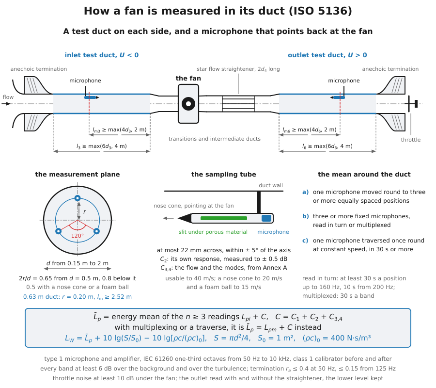
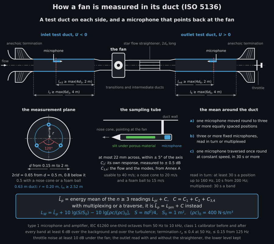
Clause 8 turns the readings into a level and the level into a power. The positions are energy-averaged and the combined correction $C$ added (Eqs 9 and 10), a multiplexed or traversed level takes the correction directly (Eq. 11), and the plane-wave relation does the rest (Eq. 12):

The three corrections are of different kinds. $C_1$ is the microphone’s free-field correction, taken from the manufacturer’s data. $C_2$ is the frequency response of the shield at normal incidence, measured on the individual tube or cone in a plane-wave field to within ±0.5 dB (clauses 5.3.3.2 c) and 5.3.4.2); the standard tabulates neither, so both are inputs here, per band or as a scalar. $C_{3,4}$, the combined mean flow velocity and modal correction, is the one the standard computes. For the sampling tube it is a polynomial in the mean flow velocity $U$ at the microphone, in metres per second, negative on the inlet side and positive on the outlet side (clause 5.3.3.4, Eq. 7):

with the coefficients $a_i$ tabulated in Annex A per one-third-octave band and per range of duct diameter (Tables A.1 to A.6), an empty cell counting as zero. The tables are normative for 50 Hz to 10 kHz and $|U|\le 40$ m/s, and their footnote adds two informative extensions that do not compose: the 50 Hz to 10 kHz rows also hold from 40 m/s to 60 m/s, while the 12.5 kHz to 20 kHz rows sit under a band header of their own that reads $|U|\le 40$ m/s and get no velocity extension, so sound_power_in_duct() refuses a velocity past 40 m/s as soon as a band above 10 kHz is asked for. For the nose cone and the foam ball no modal data exist, and clause 5.3.4.3 replaces the polynomial by the frequency-independent convective term of Eq. 8, $C_{3,4}=10\lg [1/(1-U/c{)}^2]$, where $c$ is the speed of sound in the test duct; clause 5.3.4.3 prints 340 m/s “under normal conditions”, which is what flow_modal_correction() uses on its own, while a whole determination knows the duct air and evaluates Eq. 8 with the $c$ that temperature gives, up to 0.08 dB away over the range of clause 1.1. The same sign convention applies, so it is positive on the outlet side and negative on the inlet side, a few tenths of a decibel at the velocities those shields are allowed (15 m/s for the foam ball, 20 m/s for the nose cone, clause 1.1).

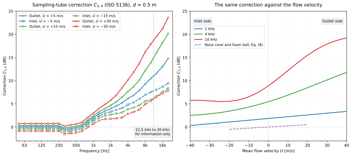
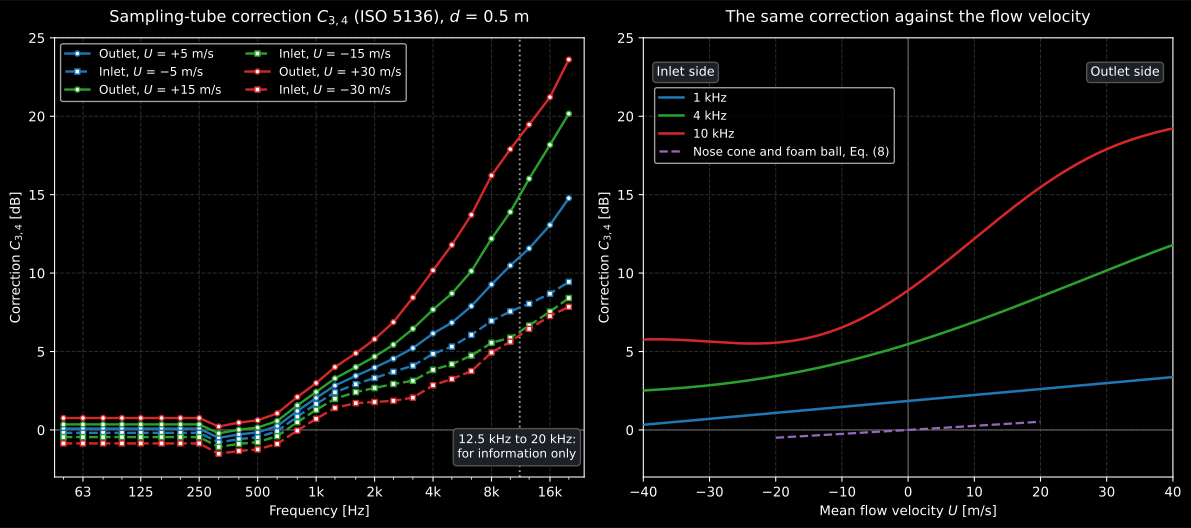
What the sampling tube costs and where. In a 0.5 m duct the correction stays within 1.6 dB of zero below 500 Hz, where the duct carries plane waves, and climbs to 10 dB and more above 4 kHz, where the higher-order modes reach the microphone from every direction and the slit tube, which listens along its axis, hears less of them. The polynomial is not odd in $U$: the same 30 m/s corrects the outlet side by 24 dB at 20 kHz and the inlet side by 8 dB, because the flow carries the modes towards the microphone on one side and away from it on the other. The omni-directional shields have no modal correction at all, only the convective term, which is why they are confined to the low velocities of clause 1.1.

import matplotlib.pyplot as plt
import numpy as np
from phonometry import emission

# A 0.5 m test duct on both sides of the fan: U > 0 on the outlet side,
# U < 0 on the inlet side, the nominal one-third-octave bands of the standard.
bands = np.array([50, 63, 80, 100, 125, 160, 200, 250, 315, 400, 500, 630, 800,
                  1000, 1250, 1600, 2000, 2500, 3150, 4000, 5000, 6300, 8000,
                  10000, 12500, 16000, 20000], dtype=float)
fig, (axf, axu) = plt.subplots(1, 2, figsize=(12.5, 5.6))
for speed in (5.0, 15.0, 30.0):
    for sign, style, side in ((1.0, "-", "Outlet"), (-1.0, "--", "Inlet")):
        c34 = emission.flow_modal_correction(bands, sign * speed, 0.5)
        axf.semilogx(bands, c34, style, marker="o",
                     label=f"{side}, U = {sign * speed:+.0f} m/s")
axf.set(xlabel="Frequency [Hz]", ylabel="Correction C3,4 [dB]")
axf.legend()

# The same correction against the flow velocity, and Eq. 8 for the nose cone.
speeds = np.linspace(-40.0, 40.0, 161)
for band in (1000.0, 4000.0, 10000.0):
    c34 = [float(emission.flow_modal_correction([band], u, 0.5)[0]) for u in speeds]
    axu.plot(speeds, c34, label=f"{band / 1000:g} kHz")
cone_speeds = np.linspace(-20.0, 20.0, 81)
cone = [float(emission.flow_modal_correction([1000.0], u, 0.5, shield="nose-cone")[0])
        for u in cone_speeds]
axu.plot(cone_speeds, cone, "--", label="Nose cone, Eq. 8")
axu.set(xlabel="Mean flow velocity U [m/s]", ylabel="Correction C3,4 [dB]")
axu.legend()
plt.show()

The example is a 630 mm axial fan measured on its outlet test duct with a sampling tube, at a mean flow velocity of 12 m/s, about 3.7 m³/s. The three positions are read in the 24 bands from 50 Hz to 10 kHz; the microphone’s free-field correction and the sampling tube’s own response come from their calibration sheets, both growing towards the top of the range.

import numpy as np
from phonometry import emission

freqs = np.array([50, 63, 80, 100, 125, 160, 200, 250, 315, 400, 500, 630, 800,
                  1000, 1250, 1600, 2000, 2500, 3150, 4000, 5000, 6300, 8000,
                  10000], dtype=float)
# The mean in-duct spectrum of the fan (dB re 20 uPa): the broadband hump of
# an axial fan around 250 Hz to 500 Hz, and the blade-passage tone of six
# blades at 1 450 r/min, 145 Hz, in the 160 Hz band.
mean = np.array([78.0, 79.5, 81.0, 82.5, 84.0, 88.0, 85.5, 86.0, 86.5, 86.0,
                 85.0, 84.0, 83.0, 82.0, 80.5, 79.0, 77.5, 76.0, 74.0, 72.0,
                 70.0, 67.5, 65.0, 62.0])
# Three circumferential positions 120 degrees apart, each a few tenths off it.
spread = np.array([[0.4], [-0.3], [-0.1]]) + 0.3 * np.sin(
    np.arange(freqs.size) * np.array([[1.0], [1.7], [2.3]]))
levels = mean + spread                                   # shape (3, 24)
c1 = np.array([0.0] * 19 + [0.1, 0.2, 0.4, 0.7, 1.1])    # microphone, dB
c2 = np.array([0.0] * 11 + [0.2, 0.3, 0.5, 0.6, 0.8, 1.0, 1.2, 1.5, 1.9,
                            2.3, 2.8, 3.4, 4.0])         # sampling tube, dB

duct = emission.sound_power_in_duct(
    levels, freqs, duct_diameter=0.63, flow_velocity=12.0,
    shield="sampling-tube", microphone_correction=c1, shield_correction=c2,
    temperature=20.0, static_pressure=101.325,
)
print(round(float(duct.mean_pressure_level[5]), 1))       # 87.9 dB at 160 Hz
print(round(float(duct.flow_modal_correction[13]), 2))    # C3,4 = 2.31 dB at 1 kHz
print(round(float(duct.combined_correction[23]), 1))      # C = 18.0 dB at 10 kHz
print(round(float(duct.sound_power_level[5]), 1))         # LW = 83.0 dB at 160 Hz
print(round(duct.sound_power_level_a, 1))                 # LWA = 89.7 dB(A)
print(round(duct.duct_area, 3), round(duct.characteristic_impedance, 1))  # 0.312 m2, 413.3 N s/m3

duct.plot()   # in-duct LW spectrum, LWA in the title (needs matplotlib)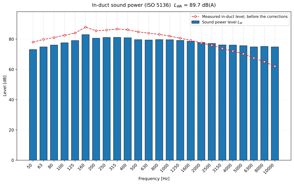

The bars are $L_W$ per band, the dashed line the level the sampling tube read before any correction. At the low end the two differ by 4.93 dB: the area term $10\lg S=-5.06$ dB for the 0.312 m² duct, and the $-0.14$ dB of the impedance term, which widens the gap rather than closing it because Eq. (12) subtracts it, less the 0.27 dB that $C_{3,4}$ already adds at 12 m/s even in the plane-wave bands. From 1 kHz up the corrections take over, until at 10 kHz the combined correction reaches 18 dB (4.0 dB of tube response, 12.9 dB of $C_{3,4}$ and 1.1 dB of microphone correction) and the power exceeds the reading by 13 dB. A spectrum read in a duct without these corrections is not the fan’s spectrum.

import matplotlib.pyplot as plt

# duct is the InDuctSoundPowerResult computed above. One line:
duct.plot()
plt.show()

# By hand: the LW bars with the uncorrected in-duct level beside them.
positions = np.arange(freqs.size)
fig, ax = plt.subplots(figsize=(10, 6.3))
ax.bar(positions, duct.sound_power_level, width=0.7, label="Sound power level LW")
ax.plot(positions, duct.mean_pressure_level, "o--",
        label="Measured in-duct level, before the corrections")
ax.set_xticks(positions)
ax.set_xticklabels([f"{f:g}" for f in freqs], rotation=45, ha="right")
ax.set_xlabel("Frequency [Hz]")
ax.set_ylabel("Level [dB]")
ax.set_title(f"In-duct sound power (ISO 5136)  LWA = {duct.sound_power_level_a:.1f} dB(A)")
ax.legend()
plt.show()

Two things in that determination are worth reading off the result rather than assuming. The first is the sign of $U$. The same three spectra read on the inlet duct of the same fan, at the same 12 m/s, carry a smaller correction, 1.39 dB instead of 2.31 dB at 1 kHz, and come out 1.6 dB(A) lower:

inlet = emission.sound_power_in_duct(
    levels, freqs, duct_diameter=0.63, flow_velocity=-12.0,
    microphone_correction=c1, shield_correction=c2,
)
print(round(float(inlet.flow_modal_correction[13]), 2))   # 1.39 dB at 1 kHz
print(round(inlet.sound_power_level_a, 1))                # 88.1 dB(A)

The second is what the omni-directional shields do not correct. A nose cone at the same 12 m/s takes the convective 0.31 dB of Eq. 8 in every band and nothing else, so the same readings give 86.6 dB(A), 3 dB less than through the sampling tube. The readings are reused unchanged only to isolate what the correction does; a nose cone in that duct would not read them. It is omni-directional, so it hears the higher-order modes the slit tube turns away from, and more of the turbulence, and its in-duct level would come out higher, which is why the standard warns in clause 5.3.4.3 that the level obtained with a nose cone or foam ball “is expected to be higher than the true sound power level”. The missing modal correction is the reason the two shields are limited to low velocities and the sampling tube is preferred (clause 4, NOTE 5).

The same NOTE 5 also says the uncertainties of Table 2 “refer to the sampling tube only and can be expected to increase for other shields”, and it puts no number on the increase. So the reproducibility a nose cone or a foam ball result carries is the sampling tube’s, which makes it a lower bound rather than that shield’s own figure, and the call says so with a SoundPowerWarning rather than leave it to be read off a table.

cone = emission.sound_power_in_duct(
    levels, freqs, duct_diameter=0.63, flow_velocity=12.0,
    shield="nose-cone", microphone_correction=c1,
)
print(round(float(cone.flow_modal_correction[0]), 2))     # 0.31 dB, every band
print(round(cone.sound_power_level_a, 1))                 # 86.6 dB(A)

The function returns an InDuctSoundPowerResult with the band $L_W$ (sound_power_level), the A-weighted total of Annex C (sound_power_level_a), the level before and after the correction (mean_pressure_level, corrected_pressure_level), the three corrections and their sum (microphone_correction, shield_correction, flow_modal_correction, combined_correction), the uncertainty statement of the next section (reproducibility_standard_deviation, expanded_uncertainty, information_only_band) and the geometry and air it was computed with (duct_diameter, duct_area, characteristic_impedance, speed_of_sound, flow_velocity, shield). flow_modal_correction() gives $C_{3,4}$ on its own for any band, velocity, diameter and shield, and in_duct_reproducibility() the ${\sigma }_R$ of the next section.

ISO 5136 states no accuracy grade. What it states is the standard deviation of reproducibility ${\sigma }_R$ of the method, band by band, for the sampling tube (clause 4, Table 2): 3.5 dB at 50 Hz, 3 dB at 63 Hz, 2.5 dB at 80 Hz and 100 Hz, 2 dB from 125 Hz to 4 kHz, then 2.5, 3, 3.5 and 4 dB at 5 kHz, 6.3 kHz, 8 kHz and 10 kHz. These are inter-laboratory figures, the spread expected if one fan were measured in many facilities, and they include the duct end reflections, the transitions, the calibration and the sampling; they do not include the fan’s own variation with its mounting. Unless the laboratory knows better, clause 9.2 says to record twice that figure as the expanded uncertainty at 95 % coverage, and that is what the result carries:

print(duct.reproducibility_standard_deviation[[0, 13, 23]])   # [3.5 2.  4. ] dB
print(duct.expanded_uncertainty[[0, 13, 23]])                 # [7. 4. 8.] dB
print(bool(duct.information_only_band.any()))                 # False

Three caveats travel with those numbers, and the result says so where it can. Table 2 is stated for the sampling tube; clause 4 NOTE 5 expects the figures to be larger for the nose cone and the foam ball and gives no others, so a determination through those shields carries the same values and the caveat. Above 10 kHz the standard is explicit that measurements “are not considered part of this International Standard”, and only suggests the extrapolated 4.5, 5 and 5.5 dB of Table 3; the Annex A coefficients are likewise for information only there, and between 40 m/s and 60 m/s. Every band in that position is flagged in information_only_band. And the figures assume the time averages of clause 7.2.2 and no strong discrete tones (NOTE 4); a fan with a dominant blade-passage tone in a low band, like the one above, will reproduce worse than 2 dB in that band.

• Covered

  The ISO 5136:2003 in-duct determination (sound_power_in_duct): the energy average over the circumferential positions (Eq. 9) or the multiplexed level (Eq. 11), the combined correction $C=C_1+C_2+C_{3,4}$ (Eq. 10) with the Annex A polynomial of the sampling tube for 0.15 m to 2 m ducts (flow_modal_correction, Tables A.1 to A.6, verified against every cell of Table D.1) and the convective term of Eq. 8 for the nose cone and foam ball, the plane-wave relation of Eq. 12 with the duct air’s $\rho c$, the A-weighted total of Annex C over the 27 bands of Table C.1, and the reproducibility of Table 2 doubled into the 95 % statement of clause 9.2 (in_duct_reproducibility), with the bands the standard gives for information only flagged as such.

• Not covered

  The facility and the instrument are assumed qualified. The reflection coefficient of the anechoic termination (Table 5, Annex F), the directivity limits of the sampling tube (Eq. 6, Table 6), the signal-to-noise check against turbulence (Annex B, Tables B.1 and G.1), the duct geometry and transitions of clause 5.2 and the swirl angle of Annex J are checks the laboratory makes, not terms of $L_W$, and none of them is computed. $C_1$ and $C_2$ are inputs: the standard tabulates neither, only how to measure them. The informative Annexes H and I, which extend the coefficient tables below 0.15 m and above 2 m, are outside the standard’s own scope and are not implemented, so a duct outside 0.15 m to 2 m is refused.

References

Section titled “References”- Arnold, F. (1999). Experimentelle und numerische Untersuchung zur Schalleistungsbestimmung in Strömungskanälen. VDI Verlag. Fortschritt-Berichte VDI, Reihe 7, Nr. 353 (Dissertation, TU Berlin, 1998). Reference [24] of ISO 5136, the source of the combined mean flow velocity and modal correction of the sampling tube and of its Annex A coefficients.
- International Organization for Standardization. (2003). Acoustics — Determination of sound power radiated into a duct by fans and other air-moving devices — In-duct method (ISO 5136:2003). Clause 8 (Eqs 9 to 12), the corrections of 5.3.3 and 5.3.4 with the Annex A coefficients and the Annex D example, the A-weighting of Annex C and the reproducibility of Table 2 that this guide implements.