Why phonometry

phonometry is a standards-based acoustic measurement toolkit. Its differentiator is not the list of features but how they are built: every metric is implemented from the governing standard’s text, and the standard’s own reference values and acceptance limits are transcribed into the test suite and enforced in CI. This page explains that approach with a concrete case study (time weighting under IEC 61672-1:2013) and summarizes what is conformance-tested today. The time-weighting analysis was originally published in issue #38.

Design philosophy: a case study in time weighting

Standard time weighting is defined as a continuous function of time via the differential equation

$$\tau \frac{dy(t)}{dt}+y(t)=x^2(t)$$

which corresponds to a stable first-order low-pass filter with a pole in the left half-plane ($s=-1/\tau$).

	phonometry	python-acoustics
Output	Continuous time-weighted envelope (one value per sample)	Stepped output (one value every $\tau$ seconds)
Input units	Raw sound pressure (Pa); squared internally	Energetic quantity (Pa²) expected as input
Filter	Stable exponential averaging (pole at $s=-1/\tau$)	Theoretically unstable design (pole in the right half-plane) stabilized by resetting the filter state every $\tau$ seconds
Behavior	True IEC time weighting	Closer to a block integrator ($L_{eq,\tau }$)

A pole on the negative real axis corresponds to a decaying exponential impulse response ($h(t)\propto e^{-t/\tau }$), exactly what “exponential time weighting” means: past events are forgotten exponentially. A pole on the positive real axis grows without bound; block-resetting hides this but changes the measurement’s nature.

That equation is also where the reference numbers of the next section come from, which is worth doing once rather than taking Table 4 on faith. Integrate it from rest over a burst of duration $T_b$ and the envelope reaches $(1-e^{-T_b/\tau })$ of the steady value the same tone would eventually produce, so the maximum time-weighted level relative to steady state is

$${\delta }_{\text{ref}}=10\lg \left(1-e^{-T_b/\tau }\right)$$

which is IEC 61672-1:2013 Equation (7). With ${\tau }_F=0.125$ s that gives −0.98 dB at 200 ms, −4.82 dB at 50 ms, −11.14 dB at 10 ms and −20.99 dB at 1 ms: the whole “IEC target” column of Table 4, to the standard’s own rounding. CI asserts the identity for every Fast and Slow row (test_delta_ref_equation7_consistency, to within 0.15 dB), so the transcription of the table is itself checked rather than trusted.

The consequence carries the rest of this page. Because the response is a smooth function of $T_b/\tau$, a detector that really solves the equation tracks the whole column at once; a detector that averages over fixed 125 ms blocks has no $T_b$ in it at all, and can only be right where the burst happens to fill a block.

Verification against IEC 61672-1 (tone bursts)

The rigorous test for time weighting is the Tone Burst Response (IEC 61672-1, Table 4), using a 4 kHz sine burst referenced to the steady-state level.

How the check is run

Table 4 fixes the excitation but not the plumbing, so here is the plumbing. A 4 kHz sine is generated at 48 kHz for 3 s. The reference is the steady Fast level of that continuous sine, averaged over its last half second — once the integrator has settled, this is $L_A$ in the standard’s notation. The burst of the stated duration is then cut out of the same sine, so its phase and amplitude are identical to the reference tone’s, and zeros surround it. The response is the maximum of the Fast envelope of that burst, expressed relative to the reference: $10{\log }_{10}(\max \text{env}/\text{ref})$, which is the standard’s $L_{AFmax}-L_A$. Note what this does and does not verify: IEC 61672-1 states these limits for the electrical input facility over a defined range of steady levels with no overload indicated (clauses 5.9.5-5.9.6), so the numbers below verify the ballistics, not a complete instrument. The same reference values are transcribed in tests/filters/test_iec_compliance.py for F and S and for the $L_{AE}$ column.

phonometry results (Fast weighting):

Burst duration	IEC target (dB)	Class 1 limit (dB)	phonometry (dB)	Error (dB)	Status
200 ms	−1.0	±0.5	−0.98	+0.02	✅ PASS
50 ms	−4.8	±1.0	−4.82	−0.02	✅ PASS
10 ms	−11.1	±1.0	−11.14	−0.04	✅ PASS
1 ms	−21.0	+1.0 / −2.0	−20.99	+0.01	✅ PASS

python-acoustics results (Fast weighting, squared signal passed as that library requires):

Burst duration	IEC target (dB)	Class 1 limit (dB)	python-acoustics (dB)	Error (dB)	Status
200 ms	−1.0	±0.5	−0.97	+0.03	✅ PASS
50 ms	−4.8	±1.0	−3.93	+0.87	✅ PASS
10 ms	−11.1	±1.0	−10.90	+0.20	✅ PASS
1 ms	−21.0	+1.0 / −2.0	−20.90	+0.10	✅ PASS

Both libraries pass every row shown, and saying otherwise would be overstating the case — the point here is the shape of the error, not a compliance failure. phonometry stays within 0.05 dB of the Table 4 reference at every duration, under 5 % of the class 1 budget, because a continuous exponential detector has no free parameter left to get wrong. The block integrator stays inside class 1 too, but it spends 0.87 of the 1.0 dB available at 50 ms, and it spends it for a reason that is luck rather than design: how the burst happens to straddle a 125 ms block. Read the two tables together with the first column of Table 4, which tightens to ±0.5 dB for bursts of 200 ms and longer — at that end a block integrator has no margin left to lose.

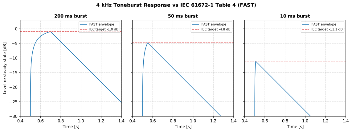
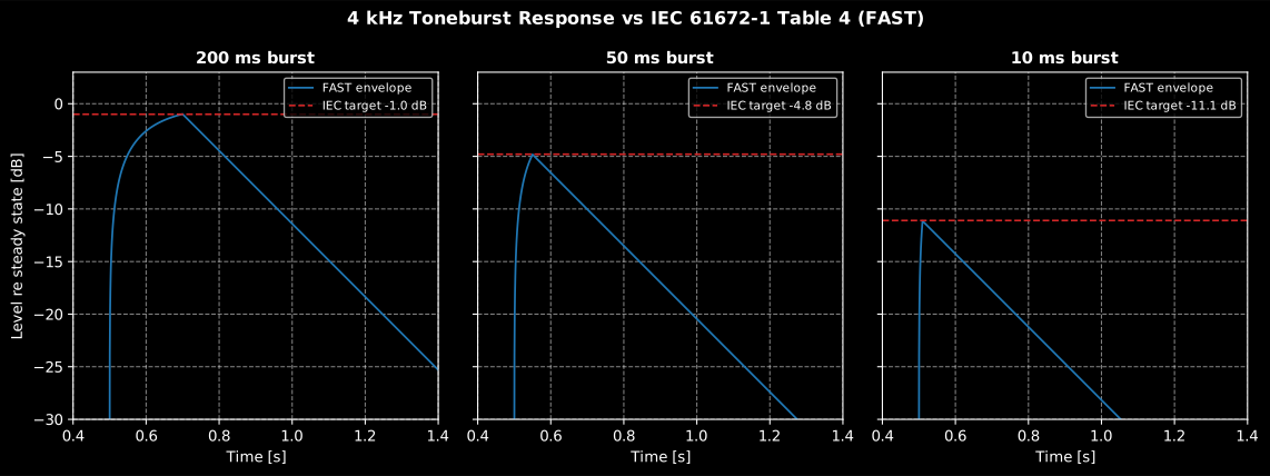
Measured Fast envelopes (blue) matching the Table 4 reference values (dashed) within 0.1 dB for 200/50/10 ms bursts.

The generator behind this figure is scripts/figures/signals.py::generate_tone_burst_iec, and it is the procedure described above with three of the Table 4 rows: it prints env_db.max() - target, which is the Error column of the first table, so the phonometry rows can be reproduced directly.

The figure fixes the burst at one place in time, which is the one thing the block integrator’s answer depends on and the exponential detector’s does not. Slide the same burst across a 125 ms block boundary and the two behave quite differently: the exponential reading is pinned at −4.82 dB whatever the alignment, a spread of 0.001 dB, while the block reading swings over 2.94 dB and spends 12 % of the alignments outside the class 1 corridor. At 200 ms, where Table 4 tightens to ±0.5 dB, the block integrator is outside the corridor for 81 % of them, because a 200 ms burst always fills at least part of a block and often fills one completely, and a full block reads the steady level, 1.0 dB above the target.

A 4 kHz tone burst slides across the boundary between two 125 ms integration blocks. The exponential Fast envelope peaks at the same level at every alignment because the burst duration enters its differential equation, while the block Leq staircase rises and falls with where the burst happens to land, and the reading-against-alignment panel builds up both traces against the shaded class 1 corridor. The second act repeats it for a 200 ms burst, where the corridor is half as wide.

Download the animation (WebM)

A 4 kHz tone burst slides across the boundary between two 125 ms integration blocks. The exponential Fast envelope peaks at the same level at every alignment because the burst duration enters its differential equation, while the block Leq staircase rises and falls with where the burst happens to land, and the reading-against-alignment panel builds up both traces against the shaded class 1 corridor. The second act repeats it for a 200 ms burst, where the corridor is half as wide.

Download the animation (WebM)

The exponential trace is flat because $10\lg (1-e^{-T_b/\tau })$ contains $T_b$ and nothing about the clock; the block trace is a picture of the alignment and nothing else. Both readings are computed here with time_weighting(x, fs, mode="fast") and with leq over consecutive 125 ms slices, against the same steady-tone reference the procedure above defines.

What this means in practice

• If you need standard-compliant Fast/Slow/Impulse envelopes (sound level meter behavior, one level per sample), use phonometry’s time_weighting.
• If you need block-averaged $L_{eq}$ per interval, that is a different, equally valid metric; you can compute it with leq over consecutive slices.
• Both approaches are useful; they just answer different questions. The discrepancy reported in issue #38 comes from comparing a continuous envelope against a block integrator, not from an implementation error.

Conformance testing across the library

A word on what a performance class is, since every verdict on this page is one. In IEC 61672-1 and IEC 61260-1 a class is not a grade of accuracy but a named tolerance corridor around a nominal response: class 1 is the narrow corridor intended for precision work, class 2 the wider one for general survey use, and both widen at the extremes of the frequency range, where they are hardest to meet. Class 0 was a narrower corridor still, in the withdrawn 1995 edition of IEC 61260, and is kept here as a voluntary extra target for the default Butterworth bank. So a PASS on this page means the computed response never leaves the corridor the standard draws; it does not mean the error is zero, and the size of the margin is the interesting number.

The tone-burst case above is not an isolated check. For each standard the library implements, the reference values and acceptance limits are transcribed from the official text into the test suite, so any regression fails CI. A sample from the metrology core:

Standard	What is verified	Test file
IEC 61672-1:2013 Table 3	A/C/Z weighting at all 34 nominal frequencies, class 1 limits, at 48 and 96 kHz	tests/filters/test_iec_weighting_table3.py
IEC 61672-1:2013 Table 4	F/S tone-burst responses (1 s to 1 ms) and the $L_{AE}$ column for sel()	tests/filters/test_iec_compliance.py
IEC 61672-1:2013 Table 5	lc_peak() one-cycle/half-cycle peak responses, class 1 limits	tests/signals/test_levels.py
IEC 61260-1:2014 Table 1	Filter-bank class 1/2 acceptance limits via verify_filter_class()	tests/filters/test_compliance.py
ISO 7196:1995 Table 2	G weighting (infrasound) at every nominal response value, 0.25–315 Hz	tests/filters/test_g_weighting.py
ISO 226:2023 Table 1 and Annex B	Equal-loudness contours and loudness levels against the Annex B tables, hearing threshold against the Table 1 $T_f$ parameters	tests/psychoacoustics/loudness/test_contours.py
ECMA-418-1:2024	TNR/PR tone prominence: critical bandwidths, proximity spacing and prominence criteria against the worked examples in clauses 10–12	tests/psychoacoustics/quality/test_tonality.py
ISO 1996-1:2016	lden(), ldn() and composite_rating_level() against hand-computed formula values	tests/environment/assessment/test_rating.py
IEC 60942:2017 Table 2	Calibrator short-term stability limits (frequency-dependent, class 1) in sensitivity()	tests/metrology/test_calibration_validation.py
IEC 61252:1993	The personal sound exposure quantities, sound_exposure() and the normalized 8 h level lex_8h()	tests/signals/test_levels.py

The same discipline applies far beyond the metrology core: today the suite runs 536 numerical conformance checks across 57 domains and 365 standards, covering psychoacoustics and speech intelligibility, room, building and materials acoustics, human and machine vibration, environmental, aircraft, rotorcraft and underwater noise, electroacoustics, broadcast loudness, industrial noise control, calibrated signal analysis and the FDTD wave solver. The full numerical report (the expected value and the value the library computes for every check, regenerated on every pull request) is published as the conformance report.

The same standards-first habit shows up below the level of whole metrics, in the numerics. Filter banks place their −3 dB points on the ANSI S1.11 / IEC 61260-1 band edges for the three architectures whose parametrization allows it, Butterworth, Chebyshev II and Bessel, the last two through corrections scipy’s raw parametrization would not apply; Chebyshev I and elliptic read the same edges as their equiripple passband edge instead, which is stated with its measured cost on Filter Banks. The default Butterworth bank is checked against the stricter class 0 of the withdrawn IEC 61260:1995 / ANSI S1.11-2004 edition as well as the current class 1. And A/C weighting stays inside class 1 tolerances up to 16 kHz at common audio rates through internal oversampling (see Frequency Weighting).

When the source is what is wrong

Transcribing a standard rather than porting somebody else’s code has a consequence that only shows up at scale: sooner or later the recomputed value and the printed one disagree, and sometimes it is the printed one that cannot be right. A worked example that contradicts its own normative clause, a constant with a digit lost in typesetting, a cross-reference pointing at the wrong equation.

Those cases are not quietly patched. Each confirmed one is written down in the standards errata with the printed edition and the exact location, what the document says, why it cannot be right, the independent evidence and the reading the library implements. Where that reading changes a number the library reports, the entry names the check or test that pins it; where it does not, because the defect is a label, a cross-reference or a table the library never reads, the entry says so instead. There are 88 of them now, across standards, guidance documents, textbooks and journal papers, each marked as reported to the issuing body or not. A defect listed there is never a defect of the method: in every case the intended reading could be established from the document itself or from physics.

That registry is the part of the approach that is hardest to fake. Code ported from another implementation inherits whatever the misprint made it do, and nothing in the port ever notices.

Where phonometry fits in the Python ecosystem

• python-acoustics was archived in February 2024 and is no longer maintained; the comparison above was run against its last released version.
• acoustic-toolbox, the community successor to python-acoustics, builds its IEC 61672-1 time and frequency weighting on pyoctaveband, the former name of this library, which since 2.1.0 is a shim over phonometry. It is only the filters that it takes from here: its own weighting.py still carries hard-coded one-third-octave A and C weighting tables.
• MoSQITo focuses on psychoacoustic sound-quality metrics and covers a good part of that ground already: Zwicker loudness, ECMA-418-2 loudness and roughness, DIN 45692 sharpness, ECMA-74 tone-to-noise and prominence ratio, and the ANSI S3.5 speech intelligibility index. phonometry implements the same family, and adds ISO 532-2 and ISO 532-3 loudness, ECMA-418-2 tonality, fluctuation strength and the Fastl & Zwicker annoyance model, none of which MoSQITo exports. What differs most is the setting. Here those metrics sit in the same conformance harness as the metrology core and compose directly with the weighting filters, ballistics, band filtering and calibration that feed them.
• pyroomacoustics simulates room impulse responses for audio and machine learning pipelines (image sources, ray tracing, beamforming, direction of arrival), and it does reach the measurement side too, with sweep-based impulse-response acquisition and an RT60 estimator. What it does not carry is the ISO 3382 parameter set. phonometry’s image-source and FDTD solvers are pinned to published closed forms, and the image-source impulse response goes through the same room_parameters analysis (EDT, T20, T30, C50, C80, D50, Ts, per band, with the ISO 3382 decay-range validity flags) as a measured one.

If your work needs numbers you can defend against a standard’s tolerance table, whether for measurement reports, environmental assessments or instrument cross-checks, that verification layer is what phonometry is for. Where the standard also fixes how the result is to be reported, the result object renders that one-page fiche itself with .report(), in English or Spanish, so the document you hand over carries the same numbers the check does. The sources behind all of it are collected in the Bibliography, every entry with a verified DOI or official publisher link.