Getting Started

phonometry is a Python toolkit for acoustic measurement, from fractional octave filter banks and frequency weighting to sound levels and standardized metrics. Every metric is verified against its governing standard: 536 numerical checks in all. Install it with pip install phonometry; the first example below filters a signal into one-third-octave bands and returns the sound pressure level of each band, and the section after it anchors those levels to a calibrator tone, which is what turns them into a measurement.

Installation

From PyPI (recommended)

pip install phonometry

Optional extras

pip install phonometry[plot]    # matplotlib, for filter response plots and result .plot() methods
pip install phonometry[perf]    # numba, faster 'impulse' time weighting
pip install phonometry[report]  # reportlab + svglib, so result .report() methods render normative PDF fiches (their figure panel needs [plot] too)
pip install phonometry[full]    # all of the above (recommended)

I recommend pip install phonometry[full]: it brings matplotlib, numba, reportlab and svglib in one go, so every feature of the library is enabled. The base install computes every metric on NumPy and SciPy alone; the only things it leaves unavailable are the figures (.plot() and the filter response plots), the normative PDF fiches (.report()) and the compiled kernel that speeds up the impulse time weighting.

One caveat about [full]: numba declares numpy<2.5, so phonometry[full] (like phonometry[perf]) resolves NumPy below 2.5 while a plain install gets the newest release. numba only makes the impulse time weighting faster, so if you would rather keep NumPy current, install phonometry[plot,report] and leave [perf] out.

From a clone

git clone https://github.com/jmrplens/phonometry.git
cd phonometry
pip install .

As a git submodule

git submodule add https://github.com/jmrplens/phonometry.git
# Then install in editable mode to use it from your project
pip install -e ./phonometry

The processing chain at a glance

Every phonometry analysis is some subset of one pipeline: take the raw signal, convert it to physical units, weight it in frequency, split it into standardized bands, smooth it in time and reduce it to metrics:

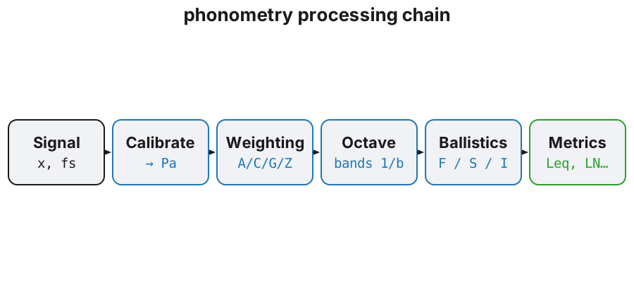
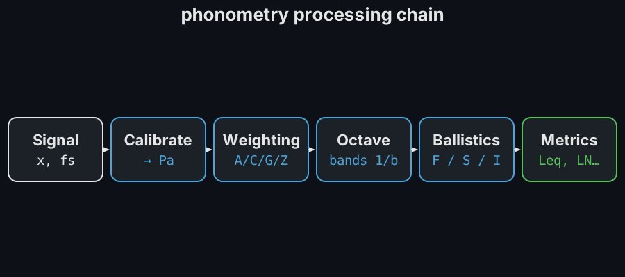
Read it as a sequence of decisions rather than a fixed recipe. Calibration comes first because everything downstream is a ratio to 20 µPa, so a wrong scale factor shifts every later number by the same amount and nothing further along can detect it. Frequency weighting is defined by IEC 61672-1 as one filter applied to the broadband signal; applying band-by-band weighting corrections after the bank instead is a shortcut that only holds for a stationary signal. The bank decides the frequency resolution, and the ballistics and the metrics decide the time behaviour — both acting on the weighted signal, in that order, because exponential time weighting squares the signal and so does not commute with anything before it.

The example in the next section runs Signal → Octave and nothing else: no calibration, so its levels are pascals by assumption rather than by measurement; no weighting, so they are Z (unweighted); no ballistics, so each band is one r.m.s. value over the whole record. “Give the samples physical meaning” below puts the first stage back, and each stage is an independent function or class you can use on its own — the guides cover them left to right (Calibration → Frequency Weighting → Filter Banks → Time Weighting → Levels).

A first analysis: one-third-octave bands (uncalibrated)

Split a signal into one-third-octave bands and read the level of each one.

import numpy as np
from phonometry import filters

fs = 48000
t = np.linspace(0, 1, fs, endpoint=False)
# Composite signal: 100Hz + 1000Hz
signal = np.sin(2 * np.pi * 100 * t) + np.sin(2 * np.pi * 1000 * t)

# Apply 1/3 octave filter bank
spl, freq = filters.octave_filter(signal, fs=fs, fraction=3)

print(f"Bands: {freq}")
# Bands: [12.589254117941678, 15.848931924611138, ..., 19952.623149688785]  (33 bands)
print(f"SPL [dB]: {spl}")
# SPL [dB]: [46.88395351 47.96774897 49.04991279 ...]  — 90.71 dB at 100 Hz and 90.95 dB at 1 kHz

The band frequencies come out as numbers, not as the labels on an analyser. IEC 61260-1 places the midband frequencies on a base-10 grid, $f_m=1000\cdot 10^{x/10b}$ with $b=3$ for one-third octaves, which is why the lowest is 12.589 Hz and the highest 19952.6 Hz. The round numbers a hand-held meter prints are the same standard’s nominal designations for the same bands: pass nominal=True and freq comes back as ['12.5', '16', …, '20k'], which is what you want on an axis or in a report, while the exact values are what you want when computing with them. There are 33 bands because the default range is 12 Hz to 20 kHz; limits=[f_min, f_max] narrows it, and narrowing it is usually worth doing — see Filter Banks for the grid.

Read the spectrum before trusting it. Two of the 33 bands hold the signal: 90.71 dB at 100 Hz and 90.95 dB at 1 kHz, both within 0.3 dB of 90.97 dB, the level of a unit-amplitude sine read as pascals ($20{\log }_{10}(0.7071/20\mu \mathrm{Pa})$). That agreement is the check that the bank is doing arithmetic you can defend; the small deficit at 100 Hz is the decimated band filter’s response at its own centre, not lost energy. Everything else on the plot is the filter bank looking at itself: 63.79 dB at 80 Hz and 65.13 dB at 125 Hz, and 53.18 dB at 800 Hz and 62.10 dB at 1.25 kHz, are the two tones leaking through the skirts of the adjacent filters, 27 to 29 dB down; the slow climb from 46.88 dB at 12.5 Hz to 54.71 dB at 50 Hz is the far stopband of those filters plus the numerical floor. The rule of thumb that follows: in a band spectrum, treat anything more than about 40 dB below the loudest band as an artefact of the analysis until a background measurement says otherwise. Filter Class Verification is the mask that fixes how far down those skirts must be.

These are not yet physical levels. octave_filter always returns $20{\log }_{10}(p_{\mathrm{rms}}/20\mu \mathrm{Pa})$, and with the default calibration it takes the numeric value of each sample to be the pressure in pascals. A unit-amplitude sine is therefore read as 0.7071 Pa rms, which is 90.97 dB — exactly right for a synthetic signal defined in pascals, and exactly wrong for a recording, whose sample values are whatever the converter and the gain staging happened to produce. There are two honest ways to get a level you can defend. Pass the pascals-per-digital-unit factor obtained from a calibrator tone, calibration=filters.LevelCalibration(factor=S) — see Calibration and dBFS — or, when the signal never had a physical scale, ask for LevelCalibration(dbfs=True) and read levels relative to digital full scale, which come out negative and cannot be mistaken for an SPL.

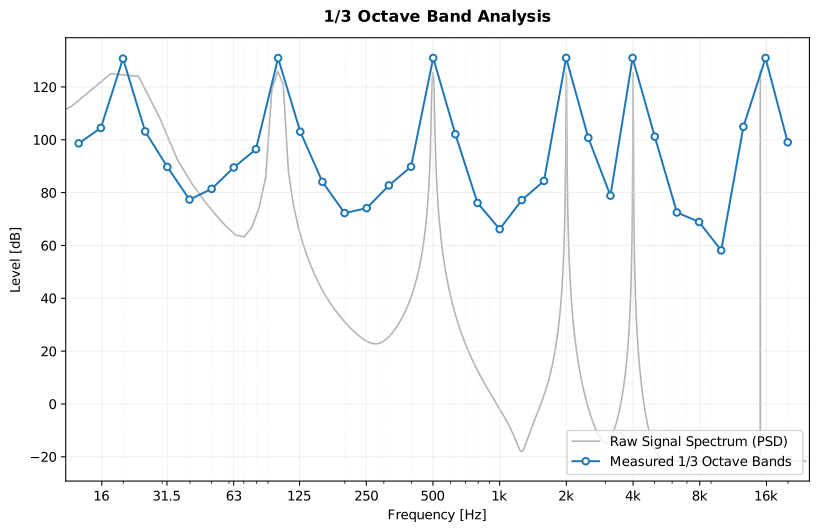
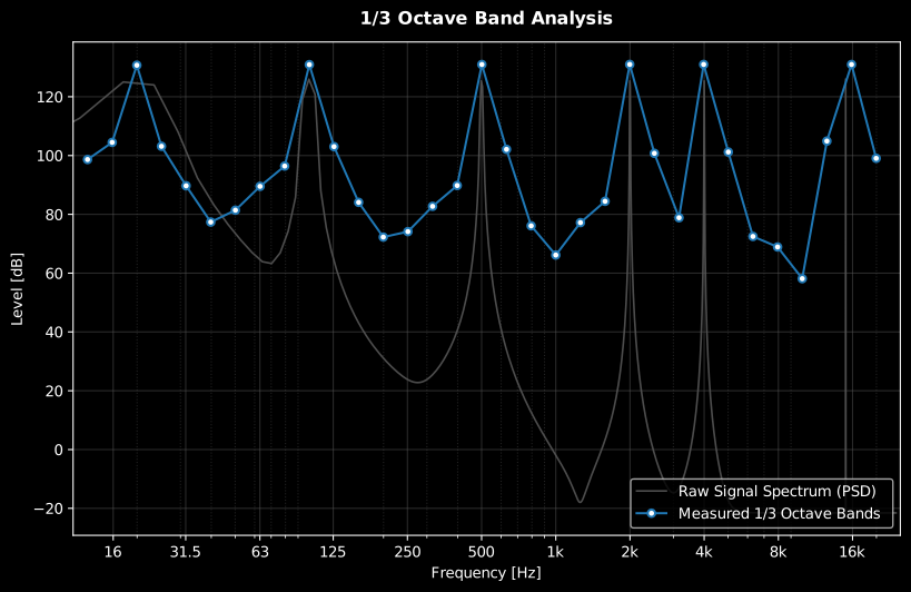
A richer example than the snippet above: six tones (20, 100, 500, 2000, 4000 and 15000 Hz) at amplitude 100, so the band levels run to about 131 dB. The grey curve is the raw-signal PSD, shifted down to share the axis.

Show the code for this figure

import matplotlib.pyplot as plt
import scipy.signal
import numpy as np
from phonometry import filters

fs = 48000
t = np.linspace(0, 5, 5 * fs, endpoint=False)
# Six tones at amplitude 100, so the bands land around 130 dB
tones = [20, 100, 500, 2000, 4000, 15000]
y = 100 * np.sum([np.sin(2 * np.pi * f * t) for f in tones], axis=0)
# Apply 1/3 octave filter bank
spl, freq = filters.octave_filter(y, fs=fs, fraction=3, limits=[12.0, 20000.0])

# Gray background: the raw-signal PSD (Welch), shifted to sit just below the
# band SPLs so both spectral shapes share one axis.
f_psd, psd = scipy.signal.welch(y, fs, nperseg=8192)
psd_db = 10 * np.log10(psd + 1e-12)
psd_db += np.max(spl) - np.max(psd_db) - 5

fig, ax = plt.subplots()
ax.semilogx(f_psd, psd_db, color="gray", alpha=0.6, label="Raw signal PSD")
ax.semilogx(freq, spl, marker="o", markerfacecolor="white",
            label="1/3 octave bands")
ax.set_xlabel("Frequency [Hz]")
ax.set_ylabel("SPL [dB]")
ax.set_xlim(11, 25000)
ax.legend(loc="lower right")
plt.show()

The same call can also draw the bank it just designed, which is what the [plot] extra is for: pass response_plot=filters.ResponsePlot(show=True) and the 33 band filters appear on one axis before the levels come back.

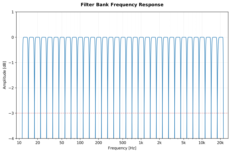
The default bank: Butterworth, order 6, one-third octave. Each curve crosses −3 dB at its own band edges, which is where the skirts of the previous paragraph come from, and the IEC 61260-1 class 1 mask is what fixes how fast they fall away.

Show the code for this figure

spl, freq = filters.octave_filter(
    signal, fs=fs, fraction=3, response_plot=filters.ResponsePlot(show=True)
)

Filter Architecture Gallery has the same plate for the other four architectures.

Give the samples physical meaning

The levels above are not a measurement, because nothing connected the numbers in the array to a pressure. That connection is a single factor $S$, the sensitivity in pascals per digital unit, and you obtain it by recording a calibrator of known level through the same microphone, preamplifier, interface and gain setting you are about to measure with. A class 1 acoustic calibrator produces 94 dB re 20 µPa at 1 kHz, which is $2\times 10^{-5}\cdot 10^{94/20}=1.0024$ Pa r.m.s. — not 1 Pa, a 0.02 dB difference that is worth getting right because it propagates into every level afterwards.

# What the acquisition chain does to the pressure. This microphone, preamplifier
# and interface together deliver 0.005 digital units per pascal; in a real
# measurement you never know this number, which is exactly what the calibrator
# is for.
chain = 0.005

# What the calibrator writes to disk: 3 s of 1 kHz at 94 dB re 20 uPa.
p94 = 2e-5 * 10 ** (94.0 / 20)                       # 1.0024 Pa RMS
calibrator = chain * np.sqrt(2) * p94 * np.sin(
    2 * np.pi * 1000 * np.arange(3 * fs) / fs
)

# ...and the measurement: the same two tones through the same chain.
recording = chain * signal

# The sensitivity is the known pressure over the RMS of the recorded tone.
cal = p94 / np.sqrt(np.mean(calibrator ** 2))
print(f"{cal:.1f} Pa per digital unit")
# 200.0 Pa per digital unit

spl, bands = filters.octave_filter(
    recording, fs=fs, fraction=3, nominal=True,
    calibration=filters.LevelCalibration(factor=cal),
)
print(f"{bands[9]} Hz: {spl[9]:.2f} dB SPL, {bands[19]}: {spl[19]:.2f} dB SPL")
# 100 Hz: 90.71 dB SPL, 1k: 90.95 dB SPL

Two things are worth noticing. The calibrated levels are the same numbers as in the first analysis, because the synthetic signal there was defined in pascals and this recording is that same field seen through a chain the calibrator has now undone — but this time they are decibels re 20 µPa because a measurement put them there, not because we assumed it. And the same recording read without the factor gives 44.93 dB in the 1 kHz band, 46.0 dB low: an uncalibrated level is not approximately right, it is off by whatever the gain staging happened to be.

In practice you do not divide by hand. metrology.sensitivity(calibrator, target_spl=94.0, fs=fs) returns the same factor and, on the way, checks the recorded tone’s short-term stability the way IEC 60942 qualifies the calibrator itself, so a badly coupled microphone is caught here instead of silently corrupting every level downstream. Calibration and dBFS carries that call, the pre/post drift rule and the digital dBFS alternative for signals that never had a physical scale.

One number instead of thirty-three

A meter shows one level, not a spectrum. On a calibrated signal that level is one line, because the A weighting and the energy average are both defined on the broadband pressure:

weighted = filters.weighting_filter(cal * recording, fs, curve="A")
laeq = 10 * np.log10(np.mean(weighted ** 2) / (2e-5) ** 2)
print(f"LAeq = {laeq:.2f} dB(A)")
# LAeq = 91.03 dB(A)

The unweighted level of the same second is 93.98 dB: A weighting takes almost 3 dB off, essentially all of it from the 100 Hz tone, which the curve attenuates by about 19 dB. signals.laeq(recording, fs, calibration_factor=cal) is the one-line form of the two lines above and applies the weighting internally, so never A-weight the signal first and then pass it to a level function — that weights it twice. The Fast and Slow envelopes, $L_{AE}$, $L_{Cpeak}$ and the percentile levels are the same kind of call: Time Weighting and Integrated and Statistical Levels have them, and Build a sound level meter runs the whole chain from a calibrator tone to all of them on one page.

Analyzing an audio file

A real measurement is two recordings, not one, and the conditions under which they are made decide what the levels are worth:

• Same chain, nothing touched in between. Record the calibrator tone first, then the measurement, through the same microphone, preamplifier, interface and gain. Lock the gain before the calibrator tone and never move it again: the factor is only valid while the chain stays as it was calibrated, and a touched gain knob is a larger error than any drift.
• Keep peaks 10–12 dB below full scale, and switch off everything automatic. Automatic gain control, noise suppression, limiting and interface EQ all change the level as a function of the level, so a processed sample can no longer be turned into a sound pressure level. A clipped one cannot either.
• Record at 48 kHz or more. At 44.1 kHz the bands above $f_s/2$ are dropped: the bank returns 32 bands ending at 15848.9 Hz instead of the 33 ending at 19952.6 Hz shown above, and says so with a PhonometryWarning.
• Repeat the calibrator check at the end. The pre/post difference is the drift bound for everything captured in between, and a common criterion invalidates the series when it exceeds 0.5 dB.

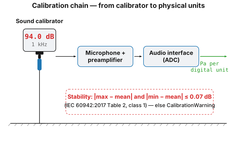
The first of the two recordings: the calibrator coupled onto the capsule at 94.0 dB / 1 kHz, through the same preamplifier and interface as the measurement that follows, producing the pascals-per-digital-unit factor everything downstream depends on.

import numpy as np
from scipy.io import wavfile
from phonometry import filters

# Both files come from the same chain, in this order, with nothing touched.
fs, calibrator = wavfile.read("calibrator.wav")
fs, signal = wavfile.read("measurement.wav")

# wavfile.read returns (samples, channels); the bank expects (channels, samples)
if calibrator.ndim > 1:
    calibrator = calibrator[:, 0]
if signal.ndim > 1:
    signal = signal[:, 0]        # measurement microphone on channel 1

# Sensitivity in pascals per digital unit, from the 94 dB calibrator tone.
# metrology.sensitivity(calibrator, target_spl=94.0, fs=fs) is the library call,
# and it validates the tone's stability as well.
cal = 2e-5 * 10 ** (94.0 / 20) / np.sqrt(np.mean(calibrator.astype(float) ** 2))

spl, freq = filters.octave_filter(
    signal, fs=fs, fraction=3, nominal=True,
    calibration=filters.LevelCalibration(factor=cal),
)

Reduce a multichannel file to the channel you measured with, or transpose it. The guard above is not decoration: wavfile.read returns a (samples, channels) array, and the bank reads a 2D array as (channels, samples). Pass a stereo file as it comes and nothing raises — a 2400-sample stereo array returns an spl of shape (2400, 33), one spectrum per pair of samples, and a one-second file takes minutes to produce meaningless numbers. See Multichannel and Performance for the convention, and for the case where several calibrated channels are analysed at once, each with its own sensitivity.

Integer audio is cast, not rescaled. wavfile.read output runs without an error because integers are converted to float64 internally, but an int16 sample of +32767 enters the bank as 32767.0 rather than 1.0. Every level therefore comes out $20{\log }_{10}(32768)=90.3$ dB above the same signal read as float — measured, a unit-amplitude 1 kHz sine peaks at 90.95 dB and the same sine written to int16 peaks at 181.26 dB. Divide by the full-scale value (signal / 32768.0 for int16) before analysing, or let the calibration step absorb it: a sensitivity determined from a calibrator recording in the same integer format already carries the factor. Mixing the two — a float-read calibrator and an integer-read measurement, or the reverse — is wrong by 90 dB with no symptom. The rules are in Calibration and dBFS.

One number per band, over the whole file. octave_filter returns a single r.m.s. level per band for the entire array, with the mean removed first (detrend=True); it answers “how much energy was in each band during this recording”, which is the right question for a steady source and the wrong one for anything that changes. A pass-by, a machine that cycles or a room that someone walks through comes back as an energy average nobody asked for. If the level moves during the record, slice the signal and call the bank per slice, or take the standard route and use the exponential Fast/Slow ballistics that a sound level meter shows; mode="peak" gives the band peak instead of the average, and a band peak is not $L_{Cpeak}$. There is a floor on the other side too: a band filter needs several cycles of its own centre frequency to settle, so a one-second record says very little about the 12.5 or 16 Hz bands however many digits come back.

Where to go next

The octave analysis above uses phonometry.filters, one of eighteen import namespaces. The documentation groups them into ten areas, one per sidebar topic, from psychoacoustics and room, building and vibration acoustics to environmental, aircraft and underwater noise, electroacoustics and FDTD wave simulation. Every result object exposes a one-line .plot(language="en"|"es") figure and, where a standard defines a reporting format, a .report() method that renders the normative PDF fiche.

• Build a sound level meter: the same chain run end to end, from the calibrator tone to $L_{AF}(t)$, $L_{Aeq}$, $L_{AE}$, $L_{Cpeak}$, the percentile levels and the class check of every stage
• All guides: the map, every guide grouped by topic with a line on each
• Glossary: a symbol, its unit, its defining clause and the guide that computes it
• Filter Architecture Gallery: choose an architecture and inspect responses
• Calibration and dBFS: get real-world SPL values
• Why phonometry: the conformance-first design philosophy
• Conformance report: the expected and computed value of all 536 checks
• API Reference: every parameter of every function
• Bibliography: the books and papers behind every guide, each with a verified link