Reading and writing measurement audio
Standards: EBU Tech 3285ITU-R BS.2088RFC 9639ITU-R BS.1770Key references: Lipshitz et al. 1992
A measurement WAV is only interpretable together with three things the
samples do not carry: the sample rate, the calibration that turns digital
full scale into pascals, and the provenance that says where and when the
recording was made. phonometry.io treats all of that as part of the file’s
meaning. read() returns a Signal (samples plus rate, calibration,
channel labels and bext provenance in one immutable object), and every
function on this page follows the same defaults: the native sample rate is
kept, channels are never mixed down, and no sample is ever normalized,
because each of those “conveniences” silently destroys the level or the
timing a measurement depends on.
The type is phonometry.io.Signal. Write it io.Signal after
from phonometry import io, or phonometry.Signal, which is the same class:
the top level publishes it because seven packages accept one, and those are
the two supported spellings. The module it is defined in is private, and
reaching into it gets the same object back, with nothing promising it will
stay reachable that way.
The base install (NumPy and SciPy alone) reads the whole linear WAV family
that measurement equipment writes: PCM at any depth including 24-bit,
IEEE float, WAVE_FORMAT_EXTENSIBLE with its channel mask, BWF bext
metadata, and RF64/BW64 recordings past 4 GiB. The [audio] extra adds
FLAC, AIFF, Ogg Vorbis, Opus, MP3 and the compressed WAV codecs some meters
use for listening copies. Nothing metrological requires the extra.
Reading a measurement
Section titled “Reading a measurement”read() takes a path and returns the Signal. The file here is written
first so the page runs; in a real workflow it comes from the instrument.
import numpy as npfrom phonometry import io
fs = 48000# recording: a stand-in for the sound level meter's WAV, synthesized so#   the guide runs; in a real measurement this file comes from the meter.rng = np.random.default_rng(11)recording = 0.02 * rng.standard_normal(10 * fs)io.write("measurement.wav", recording, fs, subtype="PCM_24")
sig = io.read("measurement.wav")print(sig.fs, sig.n_channels, f"{sig.duration:.1f} s")    # 48000 1 10.0 sprint(sig.source.format_name, sig.source.bit_depth)       # PCM 24
The object stands in for the bare array anywhere: np.asarray(sig) yields
the samples (1-D for one channel, (channels, samples) for several), so
every (x, fs, ...) function of the library already takes it in place of
the array, with the rate still passed alongside. Much of the library goes
further and takes the Signal itself (the object already knows its rate and
its calibration), and asking you to repeat either is asking for a
transcription error. The object supplies the rate when fs is omitted, and
an explicit fs that disagrees with it raises rather than being arbitrated. That covers the level
functions (leq, laeq, ln_levels, sel, lc_peak, sound_exposure
and lex_8h), the filters (octave_filter, weighting_filter,
time_weighting, linkwitz_riley, parametric_eq, and the block-processing
objects OctaveFilterBank, WeightingFilter, TimeWeighting and
ParametricEQ), and the estimators of signals: spectra
(power_spectral_density, cross_spectral_density,
coherent_output_spectrum, multitaper_psd, miso_coherence),
time-frequency (spectrogram, zoom_fft), correlation and delay
(correlation, time_delay, impulse_response_delay,
align_impulse_responses), envelope (envelope, envelope_spectrum),
cepstrum (cepstrum, lifter, echo_detection),
time_synchronous_average, regularized_inverse_filter, resample_signal
and fractional_delay, together with the data-qualification tests of
metrology (stationarity_test, level_crossing_rate, peak_statistics).
A calibrated Signal is processed in pascals. That is one rule but not one
unit: what the calibration buys depends on what the call hands back.
| What the call returns | Units under a calibrated Signal |
|---|---|
A waveform: weighting_filter, linkwitz_riley, parametric_eq, envelope, time_synchronous_average, resample_signal, fractional_delay, align_impulse_responses | Pa |
A squared envelope: time_weighting | Pa² |
A level: octave_filter, OctaveFilterBank, and the level functions | dB SPL re 20 µPa |
A spectral density: power_spectral_density, cross_spectral_density, coherent_output_spectrum, multitaper_psd, spectrogram, miso_coherence | Pa²/Hz, or Pa² under scaling='spectrum' |
A correlation: correlation | Pa² |
An amplitude spectrum: zoom_fft, envelope_spectrum | Pa |
An inverse filter: regularized_inverse_filter | 1/Pa |
A waveform comes back in the type it went in as. weighting_filter,
linkwitz_riley, parametric_eq and fractional_delay return a Signal for
a Signal, and the result objects carry theirs the same way:
envelope(...).signal, time_synchronous_average(...).period_waveform,
resample_signal(...).signal at its new rate, the aligned and reference
of align_impulse_responses, and the pressure of
underwater.pile_strike_metrics. A returned Signal carries
calibration_factor=1.0 when the input was calibrated, which says the
conversion to pascals is already done, so handing it on does not apply the
factor twice. A bare array in is a bare array out.
Ratios and times are scale-free and do not move at all: every coherence,
every normalized correlation coefficient, every phase, and every delay in
seconds or samples, which is why time_delay, impulse_response_delay and
echo_detection return for a calibrated Signal exactly what they return
for the raw record. The cepstrum is the one odd case, being a log-spectrum
transform: the factor lands entirely on the zeroth quefrency and leaves every
other one untouched, so lifter shifts its two dB spectra by 20 lg of the
factor and moves nothing else. level_crossing_rate is the one that asks
something of you: its levels are compared against the samples, so for a
calibrated Signal they have to be given in pascals.
The dbfs routes are the deliberate exception: full scale is their
reference, so they ignore the factor. For the same reason, do not chain a
filter into a dBFS reading: leq(weighting_filter(sig, curve="A"), dbfs=True)
measures pascals on a scale that claims to be full-scale referenced, and comes
out 20 log10(factor) off. That is what laeq(sig, dbfs=True) is for, which
weights the raw samples before reading them.
Integer samples are scaled by exactly for a -bit container: a power of two, so the conversion to float64 is exact in binary floating point, and the same convention as libsndfile and MATLAB. The eternal 32767-versus-32768 debate is moot here for a better reason than taste: the calibrator tone is read through this same reader, so any fixed scaling constant divides out of every calibrated level, exactly.
info() answers from the headers alone: no sample is decoded, so it is
instant on a 12-hour RF64, and it still describes a compressed WAV that
read() would need the extra for:
meta = io.info("measurement.wav")print(meta.container, meta.format_name, meta.bit_depth) # WAV PCM 24print(meta.frames, f"{meta.duration:.1f} s") # 480000 10.0 sCalibrating from the calibrator take
Section titled “Calibrating from the calibrator take”The calibration guide derives
the sensitivity factor from a recording of the calibrator tone; the only
new rule here is that both files go through the same reader. Then the
factor rides on the Signal and the level functions use it on their own:
from phonometry import metrology, signals
# calibrator.wav: the 94 dB calibrator take, synthesized so the guide runs#   (tone at -10 dBFS RMS); in a real session, record your calibrator.t = np.arange(5 * fs) / fsio.write("calibrator.wav",         np.sqrt(2) * 0.316 * np.sin(2 * np.pi * 1000 * t), fs,         subtype="PCM_24")
cal_take = io.read("calibrator.wav")cal = metrology.sensitivity(cal_take, target_spl=94.0)print(f"S = {cal:.3f} Pa per full-scale unit")            # 3.172
sig = io.read("measurement.wav", calibration_factor=cal)print(f"Leq = {float(signals.leq(sig)):.1f} dB")          # 70.0
No calibration_factor argument, no fs argument at the level call: the
Signal carries both, and the two are carried under different rules. An
explicit calibration_factor still wins over the one the object carries:
the caller knows more than an object, after a re-calibration or for a
deliberate what-if. An explicit fs does not win: the rate is a fact of the
recording rather than a preference, so a value that disagrees with the
object’s raises instead of overriding it, and only a value that agrees is
accepted. A bare array is refused by name rather than guessed at by the
functions that need a rate at all, which leq does not: it integrates the
whole record, so it never had an fs argument to omit.
Both rules hold for every function in the library that consumes a recording, with four exemptions to the calibration half. Each is a case where pascals would be the wrong thing to hand the function, and each says so in its own docstring:
- Referenced to digital full scale. The EBU R 128 family
(
program_loudnessand its parts),dynamic_rangeandidle_channel_noisecount from a full-scale sine rather than from 20 µPa. Scaling their samples would move every reading by20 lg(factor)and still call it LUFS or dBFS. - Not a pressure. A whole-body vibration record is an acceleration in m/s² and a heavy-impact record is a force in newtons, so a digital-to-pascal factor is not a unit conversion either of them wants.
- Produces the factor.
metrology.sensitivityis what a factor comes from, as in the snippet above; applying one first would calibrate the calibration. - A
dbfs=Truepath, for the same reason as the first.
Everything else takes it, including the underwater metrics: their reference of 1 µPa changes where the decibel is counted from, not what unit the samples have to be in.
The same chain on a real meter’s file
Section titled “The same chain on a real meter’s file”The repository versions a real calibration take for exactly this workflow:
tests/data/audio/xl2/calibration_113_7dB.wav, recorded by an NTi Audio
XL2 sound level meter during a road traffic pass-by campaign at the
University of Antwerp (CC BY 4.0; provenance, licence and attribution in
tests/data/audio/README.md). Being an instrument, the meter wrote its
own bext chunk and declared its digital full scale in it. That
declaration plus the file’s RMS is the whole calibration chain, and it has
to land on the level the dataset publishes for this take: 113.7 dB.
import pathlib
import phonometryfrom phonometry import io, signals
# The committed take lives in the repository, so this runs from a checkout#   (or editable install); with your own meter's WAV, pass its path directly.repo = pathlib.Path(phonometry.__file__).resolve().parents[2]xl2_take = io.read(repo / "tests/data/audio/xl2/calibration_113_7dB.wav")print(xl2_take.provenance.originator)          # NTi Audio XL2 A2A-17367-E0
declaration = xl2_take.provenance.description.splitlines()[0]print(declaration)                             # 0dBFS = 129.3 dBSPLfull_scale_spl = float(declaration.split()[2])
xl2_cal = 2e-5 * 10 ** (full_scale_spl / 20)   # what 0 dBFS is in pascalsxl2_leq = float(signals.leq(xl2_take, calibration_factor=xl2_cal))print(f"Leq = {xl2_leq:.1f} dB")               # 113.7, the published level
No hand-typed sensitivity anywhere: the instrument’s file carried its own full scale, the reader surfaced it, and the published 113.7 dB came out the other end. A recording made by the same meter is calibrated with the same two lines: which is why both files going through the same reader is the one rule that matters.
The figure below is this page in one image: the same API wrote a 24-bit BWF
with its bext chunk and its calibration sidecar, read it back, and the
resulting Signal drew its calibrated waveform next to the card of what
travelled with the samples.
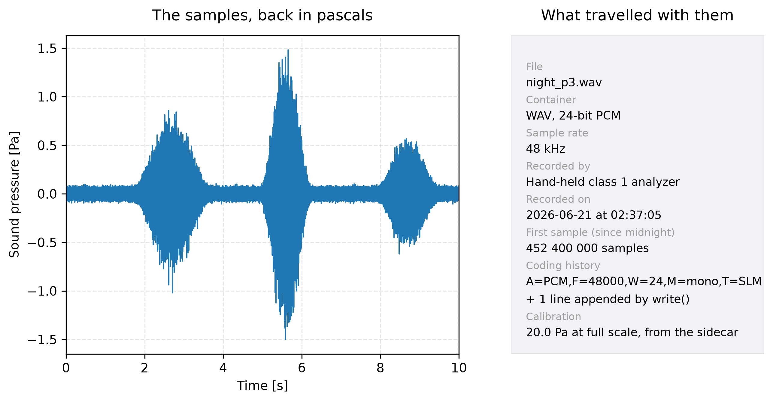
What read() returns besides samples. The waveform is in pascals because
the sidecar’s calibration was applied on read; the card is the bext
provenance of EBU Tech 3285, who recorded it, when, and at which sample
since midnight, plus the container facts and the calibration source. None
of it had to be typed back in.
Show the code for this figure
import matplotlib.pyplot as pltimport numpy as npfrom phonometry import io
fig_fs = 48000fig_rng = np.random.default_rng(2026)night = 0.0012 * fig_rng.standard_normal(10 * fig_fs)for start_s, length_s, amplitude in ((1.6, 2.2, 0.011), (4.9, 1.4, 0.020),                                     (7.8, 1.8, 0.008)):    piece = slice(int(start_s * fig_fs),                  int(start_s * fig_fs) + int(length_s * fig_fs))    envelope = np.hanning(int(length_s * fig_fs))    night[piece] += amplitude * envelope * fig_rng.standard_normal(envelope.size)
bext = io.BroadcastMetadata(    description="Night monitoring, facade position P3",    originator="Hand-held class 1 analyzer",    originator_reference="ESPHN20260621023705000012",    origination_date="2026-06-21", origination_time="02:37:05",    time_reference=(2 * 3600 + 37 * 60 + 5) * fig_fs, version=2, umid=None,    loudness_value=None, loudness_range=None, max_true_peak_level=None,    max_momentary_loudness=None, max_short_term_loudness=None,    coding_history="A=PCM,F=48000,W=24,M=mono,T=SLM",)io.write("night_p3.wav", io.Signal(data=night, fs=fig_fs,                                   calibration_factor=20.0),         subtype="PCM_24", bext=bext, sidecar=True)
night_sig = io.read("night_p3.wav")   # calibrated by the sidecarax = night_sig.plot()                 # pascals, because it is calibratedprint(night_sig.provenance.originator, night_sig.provenance.origination_time)plt.show()
The lossy warning, and the XL2 story behind it
Section titled “The lossy warning, and the XL2 story behind it”By default an NTi XL2 records WAV (compressed to 4-bit ADPCM). The manual is explicit about the intent: the compressed recording is a listening record, and linear WAV (with the Extended Acoustic Pack) is what is “required for post-processing on the PC”. The distinction matters because a lossy decoder reconstructs an approximation of the waveform: a level computed from it is not defensible as a measurement, however plausible the number looks.
So lossy sources are read, not refused (a listening copy is still worth opening), but never silently:
import soundfile as sf
# What a meter's default listening copy looks like: 4-bit IMA ADPCM in a# WAV container. Written here with soundfile to have one to read.sf.write("voice_note.wav", np.asarray(sig)[: 2 * fs], fs,         subtype="IMA_ADPCM")
note = io.read("voice_note.wav")     # emits LossyCompressionWarningprint(note.source.lossy)             # True: the fact outlives the warning
The LossyCompressionWarning fires for MP3, Ogg Vorbis, Opus and the
compressed WAV codecs alike, and source.lossy stays stamped on the signal
so the fact survives after the warning has scrolled away. Writing lossy
formats is not in the API at all: there is no measurement reason to produce
one, and a library whose job is preserving levels should not make it easy.
Two adjacent cases the module deliberately does not cover: dictaphone
AAC/M4A, where the honest route is a one-line external conversion
(ffmpeg -i note.m4a note.wav, then read("note.wav")), with the same
caveat, since AAC is lossy too; and DAQ formats that are not audio at all
(TDMS from LabVIEW hardware, UFF from modal analysis), which have their own
Python readers (npTDMS, pyuff).
Streaming an overnight recording
Section titled “Streaming an overnight recording”A night of monitoring at 48 kHz/24-bit is gigabytes; as float64 it is
~5.5 GiB per stereo hour, which no analysis needs in memory at once.
read_blocks() yields Signal blocks, each one what read() would return
for the same span: the same scaling and channel convention (base-install
seek-and-decode for linear WAV including RF64), and the same rate,
calibration, channel labels and provenance riding along. The calibration
follows the rule read() follows, so a factor passed here or found in the
sidecar makes every block present its samples in pascals to the filters and
the level functions, and no factor is applied by hand. The stateful filters
of block processing consume the
stream unchanged, and the arithmetic below takes np.asarray of what they
return, as it would of any Signal:
from phonometry import filters
weighter = filters.WeightingFilter(fs, "A", stateful=True)total_energy = 0.0total_samples = 0for block in io.read_blocks("measurement.wav", block_size=1 << 16,                            calibration_factor=cal):    weighted = np.asarray(weighter.filter(block))   # pascals, A-weighted    total_energy += float(np.sum(weighted ** 2))    total_samples += weighted.shape[-1]
streamed = 10 * np.log10((total_energy / total_samples) / (2e-5) ** 2)whole = float(signals.leq(filters.weighting_filter(sig, curve="A")))print(f"streamed {streamed:.4f} dB, whole file {whole:.4f} dB")# streamed 67.2940 dB, whole file 67.2940 dB
The two numbers are not close: they are identical, to the last bit,
because a stateful filter carries its state across block boundaries and the
stream contributes every sample exactly once. Both sides run the same default
design, since block processing no longer costs the weighting filter anything
(the weighting guide has the
detail). The same construction drives an OctaveFilterBank with
BlockProcessing(stateful=True), band by band.
Writing a BWF with its provenance
Section titled “Writing a BWF with its provenance”write() produces WAV/BWF: PCM 16, 24 (packed in-house; SciPy cannot),
32, float 32/64. It promotes to RF64 automatically past 4 GiB. Three
promises, each the opposite of a documented ecosystem default: it never
normalizes, it never resamples, and clipping is never silent: samples past
full scale on an integer subtype are saturated, counted and reported with a
ClippingWarning naming the count and the peak overshoot in dBFS. Optional
dither="tpdf" adds one-LSB triangular dither when quantising to
PCM_16 (the Lipshitz, Wannamaker and Vanderkooy prescription for
16-bit listening copies) and is refused elsewhere, because dither only adds
noise to data that faces numerical analysis rather than ears.
Provenance is first-class. A Signal’s own bext is carried by default
when it has one; a BroadcastMetadata you build is written field by field
at its EBU Tech 3285 offsets; and bext="loudness" additionally measures
the five version-2 loudness values (programme loudness, loudness range,
maximum true peak, momentary and short-term maxima) with the library’s own
ITU-R BS.1770 implementation
on the samples being written. Every written chunk’s CodingHistory is
extended, never replaced, with the EBU R98-formatted line describing this
coding step.
out = io.Signal(data=np.asarray(sig), fs=fs, calibration_factor=cal)io.write("delivery.wav", out, subtype="PCM_24", bext="loudness",         sidecar=True)
delivered = io.info("delivery.wav")print(delivered.bext.loudness_value)        # -30.85 (LUFS, measured)print(delivered.bext.max_true_peak_level)   # -20.08 (dBTP, measured)
The sidecar: how the calibration travels
Section titled “The sidecar: how the calibration travels”No audio container has a field for a microphone calibration; bext has
none, and its loudness values are programme loudness, not sensitivity. The
industry answer is proprietary companions (a meter’s report text, a
manufacturer’s project file); seismology’s answer, a standardized sidecar
beside the waveform, is the one worth copying. write(sidecar=True) (or
write_sidecar() for an existing file) puts a small versioned JSON at
<audio>.phonometry.json carrying the calibration factor, the calibrator
tone’s metadata and the channel labels, and read() applies it
automatically: an explicit argument still wins, and a sidecar written by a
newer schema or another tool is refused loudly rather than half-understood.
again = io.read("delivery.wav") # no argument this timeprint(f"{again.calibration_factor:.3f}") # 3.172, from the sidecarprint(f"Leq = {float(signals.leq(again)):.1f} dB") # 70.0: the level survived the diskThat round trip is the point of the whole page: write a calibrated signal, read it back with no arguments, and the absolute level is intact.
Conversion that keeps the measurement a measurement
Section titled “Conversion that keeps the measurement a measurement”convert() moves a file between lossless containers with everything
intact: samples at full precision (a WAV-24 to FLAC to WAV-24 round trip
returns bit-identical codes), the bext chunk carried: into FLAC it rides
in an APPLICATION block the readers here understand. The sidecar is copied
byte for byte, and one line appended to the CodingHistory naming the
coding step. Lossy targets are refused by policy. The conversion streams,
so an hour of RF64 converts in constant memory:
io.convert("delivery.wav", "delivery.flac")
flac = io.read("delivery.flac")print(flac.provenance is not None)                            # Trueprint(float(signals.leq(flac)) == float(signals.leq(again)))  # True: identical
The equality is == on floats and it holds: FLAC stores the same integer
codes, the reader scales them by the same power of two, and the archived
level is identical, not merely close.
What each install reads and writes
Section titled “What each install reads and writes”| Base install (NumPy + SciPy) | With pip install phonometry[audio] | |
|---|---|---|
| Read | WAV/BWF: PCM at any depth, IEEE float 32/64, EXTENSIBLE (channel labels), bext, cue points, RF64/BW64 | + FLAC, AIFF, Ogg Vorbis, Opus, MP3, compressed WAV (ADPCM, A-law/µ-law) |
| Write | WAV/BWF: PCM 16/24/32, float 32/64, RF64 automatic, bext, sidecar | + FLAC (PCM up to 24-bit, bext carried) |
| Stream | read_blocks on linear WAV (RF64 included) | + read_blocks on every readable format |
info() | Every WAV-family file, compressed included | + the extra formats |
The extra is python-soundfile, whose wheel bundles libsndfile under the LGPL-2.1 (dynamically linked, the same pattern as librosa and torchaudio); the base install stays BSD/MIT-only, which is why every metrological format lives there.
read() and write() parameters
Section titled “read() and write() parameters”| Parameter | Type | Default | Notes |
|---|---|---|---|
read(path) | str / Path | — | Dispatch is by leading magic bytes, not extension: a mislabelled file dispatches by what it is |
read(..., calibration_factor=) | float, optional | None | Digital-to-pascal multiplier; None takes an existing sidecar’s factor, else the signal stays in full-scale units |
write(path, x, fs) | — | — | x is a Signal (then fs may be omitted, and a disagreeing explicit one raises) or an array in (channels, samples) order |
write(..., subtype=) | str, optional | float data "FLOAT", integer data its own depth | "PCM_16", "PCM_24", "PCM_32", "FLOAT", "DOUBLE"; FLAC targets take PCM up to 24 |
write(..., bext=) | BroadcastMetadata / "loudness" | None | None still carries a Signal’s own provenance; "loudness" measures the five R 128 fields in-house (one extra pass, which is why it is opt-in) |
write(..., dither=) | "tpdf", optional | None | Only with subtype="PCM_16"; refused elsewhere |
write(..., sidecar=) | bool | False | Requires a calibrated Signal: a sidecar without a calibration would be a promise with nothing behind it |
Quick answers
Section titled “Quick answers”Why does my sound level meter’s WAV read as tiny numbers instead of pascals?
Section titled “Why does my sound level meter’s WAV read as tiny numbers instead of pascals?”Because a WAV carries no calibration: the samples come back in digital
full-scale units (±1.0), and only a calibrator take recorded through the
same chain turns them into pascals. Read the calibrator file with read(),
derive the factor with sensitivity(), and pass it as
calibration_factor=, or write it into the sidecar once and let read()
apply it from then on.
Can I compute Leq from the meter’s compressed voice-note WAV?
Section titled “Can I compute Leq from the meter’s compressed voice-note WAV?”You can make the call, and the library will answer after a
LossyCompressionWarning, with source.lossy stamped on the signal. The
number is not defensible: an ADPCM or MP3 decoder reconstructs an
approximation of the waveform, and the error is program-dependent. Use the
meter’s linear recording mode for anything that produces a level.
Do I need the [audio] extra to read my recordings?
Section titled “Do I need the [audio] extra to read my recordings?”Almost certainly not for measurements: the base install reads every linear WAV variant meters and field recorders write, including 24-bit, EXTENSIBLE multichannel and RF64 files past 4 GiB. The extra is for FLAC archives, AIFF/Ogg/Opus/MP3, and the compressed WAV listening copies, and it bundles libsndfile under the LGPL, which the base install deliberately avoids.
References
Section titled “References”- European Broadcasting Union. (2011). Specification of the Broadcast Wave Format (BWF) — A format for audio data files in broadcasting, Version 2.0 (EBU Tech 3285). The bext chunk this page reads and writes field by field: originator, the sample-accurate since-midnight time reference, CodingHistory, and the five EBU R 128 loudness values of version 2.
- International Telecommunication Union. (2023). Algorithms to measure audio programme loudness and true-peak audio level (Recommendation ITU-R BS.1770-5). The loudness algorithm behind bext="loudness": the five version-2 fields are measured by the library's own implementation on the samples being written.
- International Telecommunication Union. (2025). Long-form file format for the international exchange of audio programme materials with metadata (Recommendation ITU-R BS.2088-2). The 64-bit RF64/BW64 container an overnight recording promotes to past 4 GiB, read here through its ds64 sizes; it superseded EBU Tech 3306.
- Internet Engineering Task Force. (2024). Free Lossless Audio Codec (RFC 9639). The lossless codec this page archives to: bit-exact integer samples up to 32 bits, which is what lets a WAV-to-FLAC-to-WAV round trip return the identical codes.
- Lipshitz, S. P., Wannamaker, R. A., & Vanderkooy, J. (1992). Quantization and dither: A theoretical survey. Journal of the Audio Engineering Society, 40(5), 355-375. Why the optional dither is triangular-PDF at one LSB, why it is offered only when quantising to 16 bits, and why it stays opt-in for data that faces numerical analysis.