Psychoacoustics & Speech Intelligibility

Level metrics tell you how much sound pressure there is; psychoacoustic metrics tell you what a listener actually perceives. This page covers loudness (ISO 532-1), sharpness (DIN 45692) and the speech transmission index (IEC 60268-16).

Loudness in sones (ISO 532-1, Zwicker)

Decibels compress perception: 10 dB more reads as twice as loud, and two sounds with the same dB(A) can differ audibly depending on how their energy spreads over the ear’s critical bands. The Zwicker method models the hearing chain explicitly — outer/middle-ear transmission, critical-band analysis on the 24 Bark scale, level-dependent masking slopes — and outputs loudness N in sones, a ratio scale: 4 sones is twice as loud as 2 sones. By definition a 1 kHz tone at 40 dB SPL is 1 sone, and every +10 phon doubles the sone value.

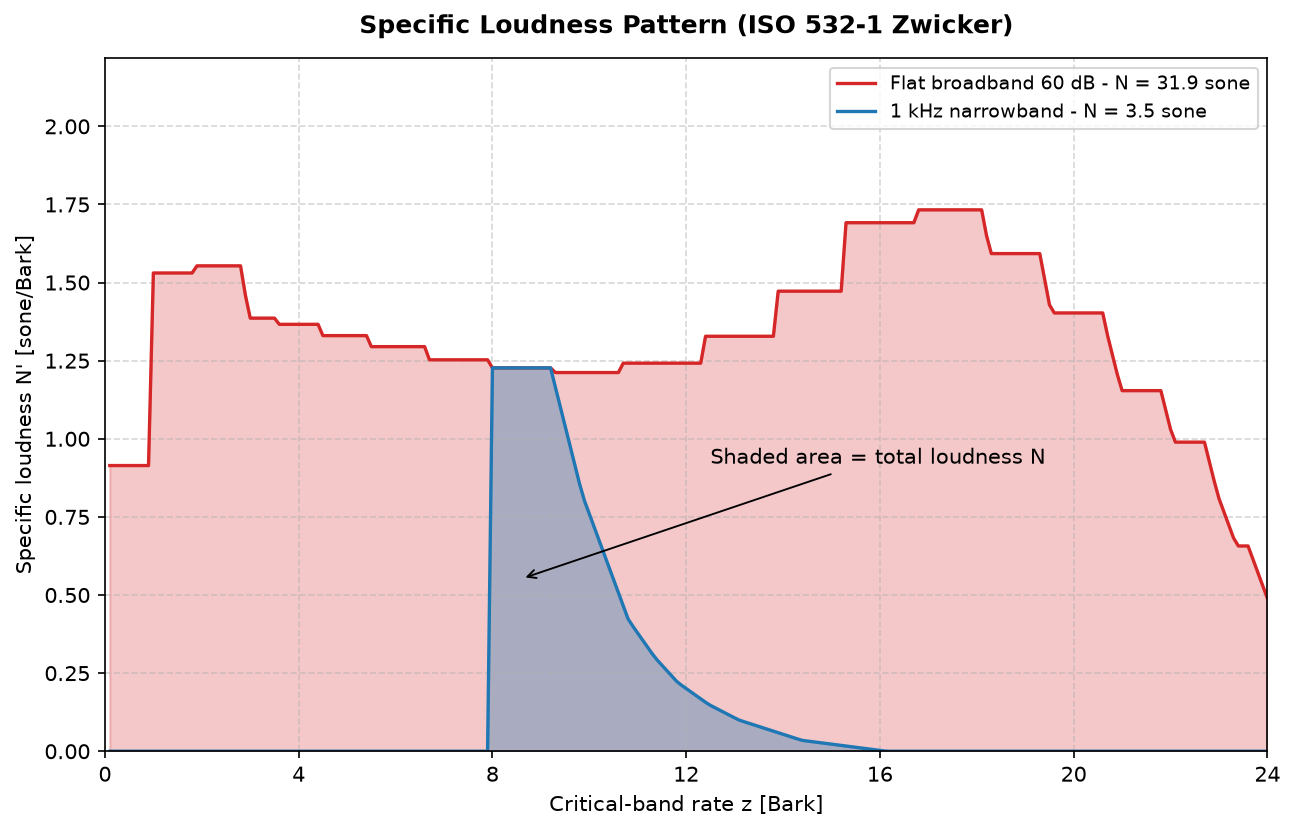
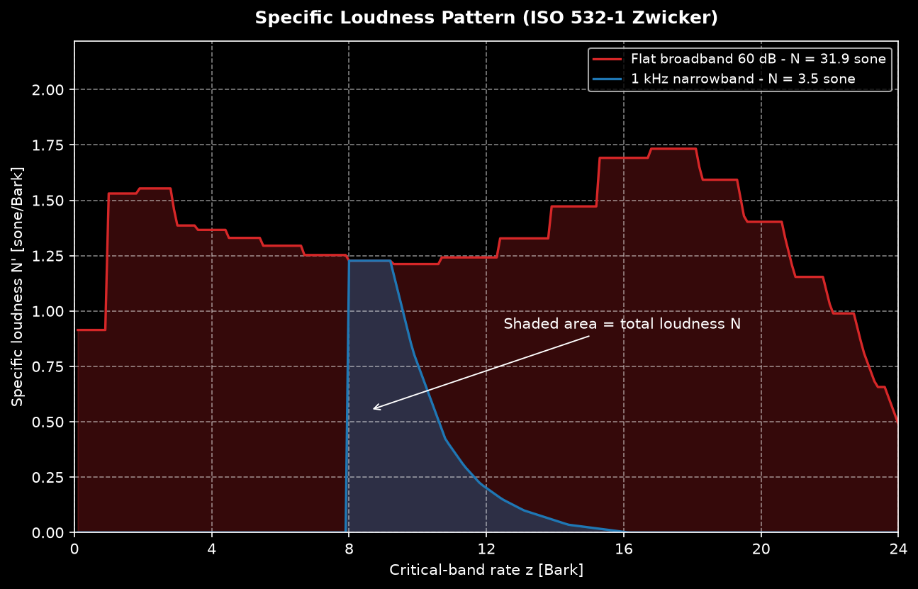
Same band level, very different loudness: energy spread over many critical bands (red) sums to far more sones than the same level concentrated in one band (blue). The area under N’(z) is the total loudness.

from phonometry import loudness_zwicker, loudness_zwicker_from_spectrum

# From a raw recording: calibration_factor scales digital units to Pa
res = loudness_zwicker(x, fs, field="free", calibration_factor=sens)
print(f"N = {res.loudness:.1f} sone  ({res.loudness_level:.0f} phon)")

# Time-varying signals: percentile loudness N5 is the reporting standard
res = loudness_zwicker(x, fs)          # stationary=False (default)
print(res.n5, res.n10, res.loudness)   # N5, N10, Nmax

# From 28 one-third-octave band levels (25 Hz .. 12.5 kHz)
res = loudness_zwicker_from_spectrum(levels_28, field="diffuse")

The implementation is a clean-room port of the standard’s normative reference program (Annex A.4): all twelve data tables are digit-exact and the full Annex B validation set runs in CI — the stationary test case reproduces the published value to every printed digit, and the tone-pulse N(t) traces stay inside the standard’s per-sample 5 % tolerance band.

loudness_zwicker() parameters

Parameter	Type	Units	Range / default	Notes
x	1D array	Pa (after calibration)	≥ 8 ms at 48 kHz	Resampled internally to 48 kHz if needed
fs	int	Hz	> 0
field	str	—	'free' (default) / 'diffuse'	Sound-field correction (Table A.5)
stationary	bool	—	default False	True: single N from the averaged spectrum
calibration_factor	float	Pa per digital unit	default 1.0	From calculate_sensitivity()

Returns a ZwickerLoudness dataclass: loudness (N, sones), loudness_level (phon), specific (N′(z), 240 bins of 0.1 Bark), and for time-varying runs n5, n10, time, loudness_vs_time (500 Hz trace).

Sharpness in acum (DIN 45692)

Two sounds can be equally loud yet one feels “sharper” — hissy, metallic — because its loudness sits higher on the Bark scale. Sharpness is the g(z)-weighted first moment of the specific loudness pattern:

$$S = k\,\frac{\int_0^{24} N'(z)\, g(z)\, z\ dz}{\int_0^{24} N'(z)\ dz}\ \text{acum}$$

with $g(z) = 1$ up to 15.8 Bark and rising exponentially beyond, and $k$ normalized so the reference sound — critical-band-wide noise at 1 kHz, 60 dB — is exactly 1.00 acum (DIN 45692 clause 6; the derived $k = 0.108$ sits inside the normative window 0.105–0.115).

from phonometry import sharpness_din

s = sharpness_din(x, fs, calibration_factor=sens)      # acum
s_aures = sharpness_din(x, fs, method="aures")          # Annex B variant

CI verifies the Table A.2 target values (0.38 acum at 250 Hz up to 2.82 acum at 4 kHz) within the standard’s 5 % / 0.05 acum tolerance.

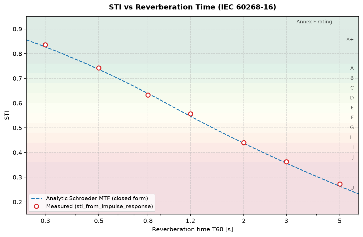
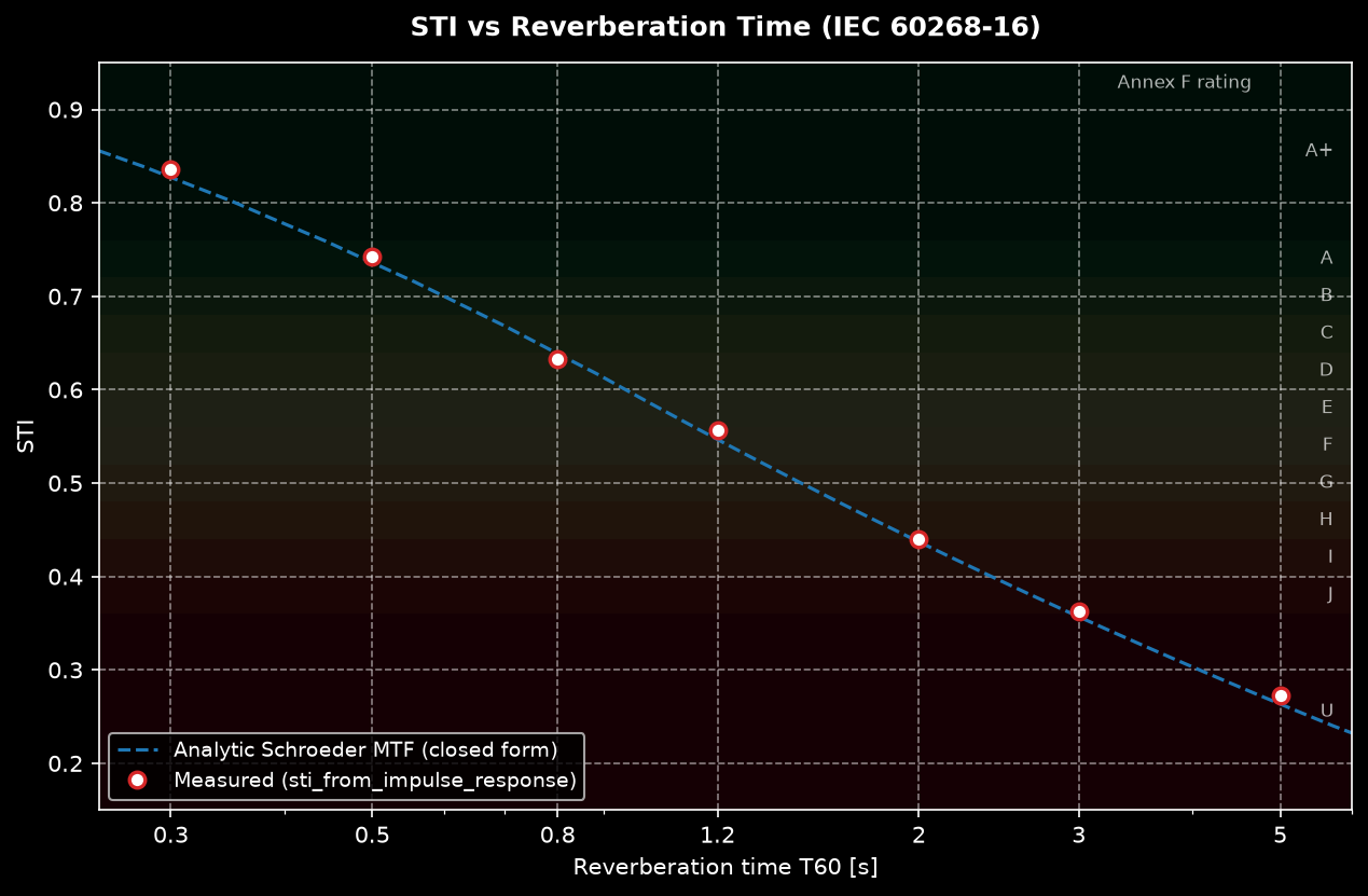
Speech Transmission Index (IEC 60268-16)

Reverberation and noise do not muffle speech uniformly — they blur its envelope: the slow (0.63–12.5 Hz) intensity modulations that carry syllables. STI quantifies how much of that modulation survives from mouth to ear, per octave band, as the modulation transfer function m(F). A delta-like channel keeps m = 1 (STI = 1); reverberation low-passes the envelope following Schroeder’s closed form, and steady noise scales it:

$$m(F) = \frac{1}{\sqrt{1 + \left(2\pi F\,\frac{T_{60}}{13.8}\right)^2}} \cdot \frac{1}{1 + 10^{-\mathrm{SNR}/10}}$$

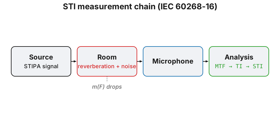
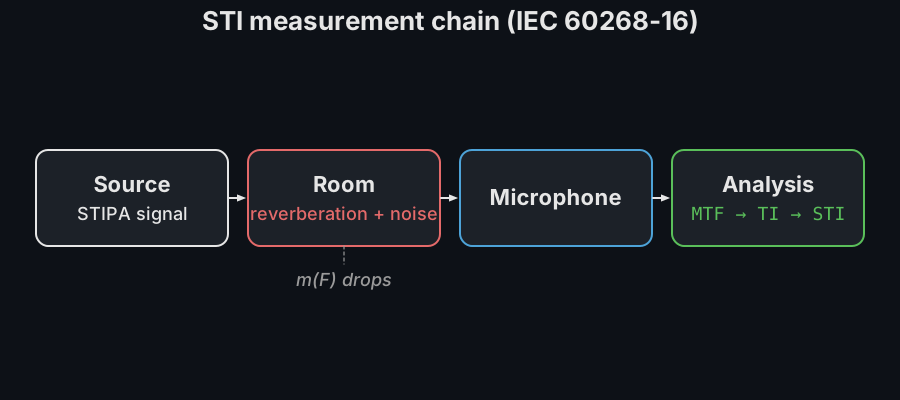
from phonometry import sti_from_impulse_response, stipa, stipa_signal

# Indirect method: from a measured room impulse response
res = sti_from_impulse_response(ir, fs, snr=25.0)
print(f"STI = {res.sti:.2f}  ({res.rating})")   # e.g. 0.62 (D)

# Direct STIPA measurement: play stipa_signal() in the room, record it
test = stipa_signal(fs, seconds=18.0, level_db=80.0)
res = stipa(recording, fs)

The implementation follows Edition 5 (2020): Edition 4’s normative PDF is the base and every Ed. 5 change is source-attributed in the code — the only numeric delta is the revised male speech spectrum of clause A.6.1. CI checks the standard’s own verification vectors: the six weighting-factor band pairs to ±0.001 STI, the m ↔ STI mapping table, the level-dependent masking control points, and Schroeder-form decays at four T₆₀ values.

sti_from_impulse_response() / stipa() parameters

Parameter	Type	Units	Range / default	Notes
ir / x	1D array	any / Pa	non-empty	IR (indirect) or STIPA recording (direct)
fs	int	Hz	> 0
snr	float or 7-vector, optional	dB	default None	Adds steady-noise degradation
level	7-vector, optional	dB SPL	default None	Enables auditory masking + reception threshold (Tables A.2/A.3)
ambient	7-vector, optional	dB SPL	needs level	Ambient noise band levels
reference	1D array, optional (stipa)	—	default None	Measured source signal instead of the nominal m = 0.55

Both return STIResult: sti, mti (7 bands), mtf (7×14 or 7×2), band_levels, rating (Annex F letter A+…U).

See Levels for tonality metrics and Theory for the underlying math.