Airport Noise (ECAC Doc 29)

Certification measures one aeroplane at one reference point on one flight; an airport study asks a different question: how loud is it there, on that street, for that departure. The ECAC Doc 29 method answers it without re-measuring anything. The aeroplane arrives as a noise-power-distance (NPD) table, a measured event level against slant distance for a handful of engine power settings; the flight arrives as a path of segments; and the method corrects the NPD baseline segment by segment for everything the tables could not know: the atmosphere on the day, the finite length of each segment, how far off to the side the receiver sits, where the engines are mounted, and the rearward lobe of a jet still on the runway.

This page covers that chain end to end, from the NPD interpolation to the ground-grid contour, and it is validated against the reference workbook of Doc 29 5th ed. Vol. 3. The certification metric these tables ultimately come from, the EPNL of ICAO Annex 16, is Aircraft noise; the physical propagation ingredients (ground effect, atmospheric absorption, barriers) are Outdoor sound propagation.

1. The noise-power-distance engine

The ECAC Doc 29 airport-noise method describes an aircraft with noise-power- distance (NPD) tables. npd_level reads the event level ($L_{Amax}$/SEL) for an arbitrary power and distance, interpolating linearly in power (Eq. 4-3) and log-linearly in slant distance (Eq. 4-4).

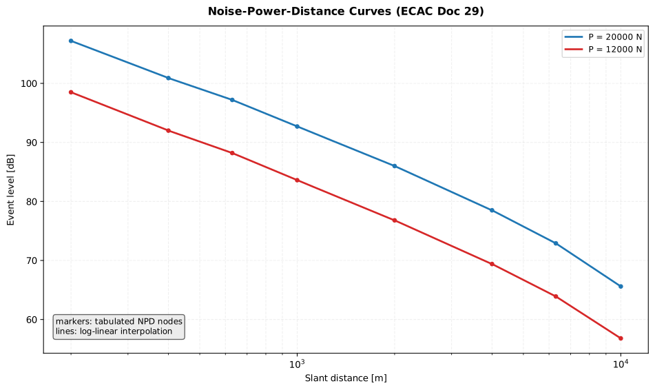
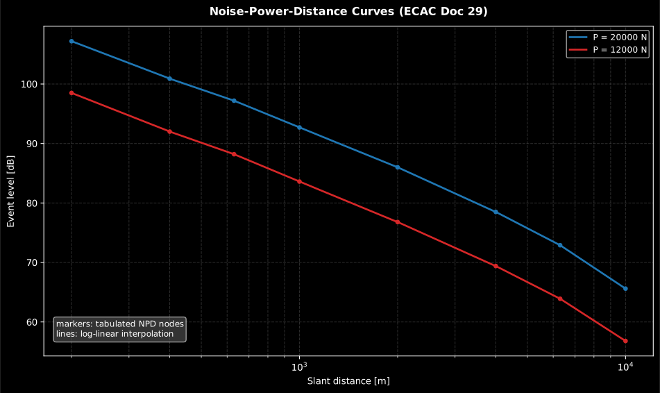
The markers are the only distances the table asserts; everything between them is the interpolation. The two curves are close to parallel — 8.7 to 9.2 dB apart over the whole range — so thrust mostly shifts the level while distance sets the shape, and the fall is 21.7 dB per decade of slant distance rather than the 20 dB of pure divergence, the excess being the reference atmosphere’s absorption. Power is interpolated linearly, not in decibels: 16 000 N reads 88.15 dB at 1 km, exactly halfway between the two tabulated rows.

Show the code for this figure

import matplotlib.pyplot as plt
from phonometry import aircraft

# A schematic NPD table: SEL vs slant distance for two thrust settings.
powers = [12000.0, 20000.0]
distances = [200.0, 400.0, 630.0, 1000.0, 2000.0, 4000.0, 6300.0, 10000.0]
levels = [[98.5, 92.0, 88.2, 83.6, 76.8, 69.4, 63.9, 56.8],
          [107.2, 100.9, 97.2, 92.7, 86.0, 78.5, 72.9, 65.6]]

fig, ax = plt.subplots()
for p in (20000.0, 12000.0):
    curve = aircraft.npd_curve(powers, distances, levels, power=p)
    line, = ax.semilogx(curve.distance, curve.level, label=f"P = {p:.0f} N")
    ax.semilogx(curve.table_distances, curve.table_levels, "o", markersize=4,
                color=line.get_color())
ax.set(xlabel="Slant distance [m]", ylabel="Event level [dB]",
       title="Noise-power-distance curves (ECAC Doc 29)")
ax.grid(True, which="both", alpha=0.3)
ax.legend()
plt.show()

from phonometry import aircraft

powers = [12000.0, 20000.0]
distances = [200.0, 400.0, 1000.0, 2000.0, 6300.0, 10000.0]
levels = [[98.5, 92.0, 83.6, 76.8, 63.9, 56.8],
          [107.2, 100.9, 92.7, 86.0, 72.9, 65.6]]
aircraft.npd_curve(powers, distances, levels, power=20000.0).plot()

This is the NPD engine underneath the method.

A tabulated NPD level is not a free-standing measurement. It is the event level of that aeroplane in steady straight flight along an infinite path, at a fixed reference condition (§2.5): sea-level pressure, the average atmospheric attenuation rates of Appendix D Table D-1, no precipitation, wind below 8 m/s, a 160 kn groundspeed for the exposure levels, and flat acoustically soft ground with the microphone 1.2 m above it. Those attenuation rates are arithmetic averages over European and American certification campaigns, so the reference day is a notional atmosphere — Doc 29 calls it the AIR-1845 atmosphere — rather than a temperature and a humidity you could quote back. Every correction in section 2 exists to undo one of those assumptions.

The tables may be used as tabulated while the site average stays inside the §2.5 envelope: air temperature below 30 °C, the product of temperature in degrees Celsius and relative humidity in percent above 500, and wind below 8 m/s. Outside it the tables themselves have to be converted by the Appendix D procedure, which this chain does not do — impedance_adjustment only rescales the levels for the specific acoustic impedance of the air, and there is no humidity argument anywhere in the chain.

Read the curves accordingly. Between the markers the level falls close to linearly against the logarithm of distance and steepens at long range as absorption accumulates; the markers are the only distances at which the table asserts anything, everything between them is the Eq. 4-4 interpolation, and everything beyond the last node is a straight-line extrapolation of the terminal slope. Do not query below the recommended 30 m floor, where a whole aeroplane stops behaving like a point source. One restriction runs under all of it: the SAE AIR 5662 lateral attenuation, and therefore the single-event chain that uses it, is derived for acoustically soft, grassy ground, so a contour drawn over water, an apron or dense urban surfaces is outside the method as published.

2. The single-event calculation

The flight arrives as a path of points, and the method cuts it into segments. path is an $(N,5)$ array:

Column	Quantity	Units
0	$x$, along the runway centre line	m
1	$y$, across it, positive to starboard	m
2	$z$, height above the aerodrome	m
3	power, the NPD power parameter	whatever the table is indexed by
4	true airspeed	m/s

$N$ points make $N-1$ segments, so every per-segment mask carries $N-1$ entries — which is why the ground-roll masks below read xs[:-1] < 1500.0 and not xs < 1500.0. Two defaults decide more than they look like they do. The speed column enters the duration correction relative to reference_speed, whose default is 82.31 m/s, the Doc 29 160 kn reference, so a path flown at exactly that speed carries no duration correction at all — which is the case in every example on this page, and varying the column is how you see the term work. And mounting= defaults to "wing": that is a property of the aeroplane rather than a modelling preference, so pass "fuselage" or "propeller" explicitly, because a propeller takes no installation correction at all and leaving the default in place gives it a directivity it does not have. Where a real type’s mounting and power units come from is The ANP fleet database.

Each segment starts from a baseline level read from the NPD table at that segment’s power and distance, and is corrected term by term:

Function	Symbol	Doc 29	What it accounts for
impedance_adjustment	${\Delta }_{\text{imp}}$	§4.2.1	the air at the aerodrome against the 409.81 N·s/m³ reference impedance of the tables
duration_correction	${\Delta }_V$	§4.5.1	the segment speed against the NPD reference speed (exposure levels only)
engine_installation_correction	${\Delta }_I(\phi )$	§4.5.3	where the engines are mounted, through the depression angle
lateral_attenuation	$\Lambda (\beta ,\ell )$	§4.5.4	ground effect and refraction for a receiver off to the side
noise_fraction	${\Delta }_F$	§4.5.6	the share of the infinite-path energy a finite segment contributes (exposure levels only)
start_of_roll_directivity	${\Delta }_{\text{SOR}}(\psi )$	§4.5.7	the rearward jet lobe behind a take-off ground-roll segment

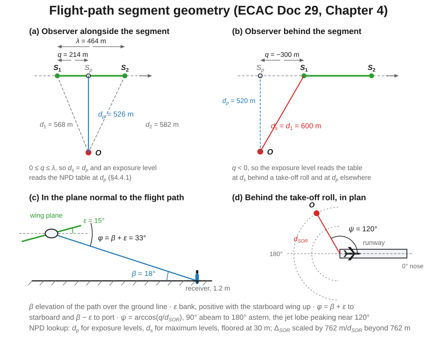
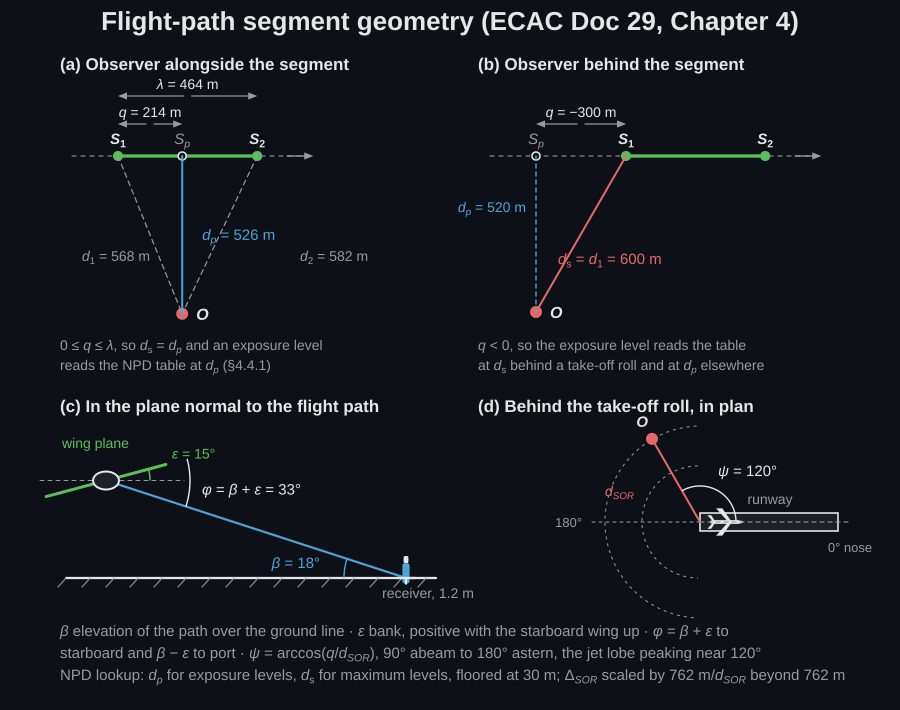
$\beta$ is the elevation angle of the propagation path above the ground line at the receiver and $\ell$ the perpendicular distance from the receiver to the ground track; $\epsilon$ is the bank angle, positive with the starboard wing up, and $\phi =\beta \pm \epsilon$ the depression angle in the aircraft frame, plus for observers to starboard and minus to port (§4.5.2). Along the track, $\lambda$ is the segment length, $q$ the distance from the segment start to the foot of the perpendicular (negative behind the segment), $d_p$ the perpendicular distance to the extended segment and $d_s$ the shortest distance to the segment itself (§4.4.1). $\psi$ is the azimuth from the nose that the start-of-roll lobe is a function of.

They assemble into a segment exposure level as

$$L_{E,\text{seg}}=[L_{E\infty }(P,d)+{\Delta }_{\text{imp}}]+{\Delta }_V+{\Delta }_I(\phi )-\Lambda (\beta ,\ell )+{\Delta }_F+{\Delta }_{\text{SOR}}$$

where the bracket is the impedance-adjusted NPD baseline of §4.2.1 and the rest is Eq. 4-8b (Eq. 4-9b behind a ground roll), and the event level is the energy sum over the segments, $L_E=10\lg \sum 10^{L_{E,\text{seg}}/10}$ (Eq. 4-11). A maximum level takes the largest segment value instead (Eq. 4-10) and drops the two terms that exist only for exposure, ${\Delta }_V$ and ${\Delta }_F$.

Their magnitudes are worth carrying, because they decide which term matters for a given receiver.

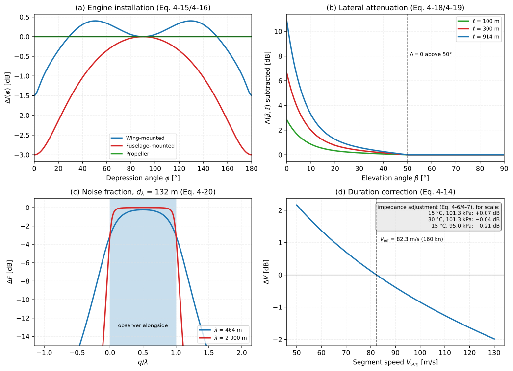
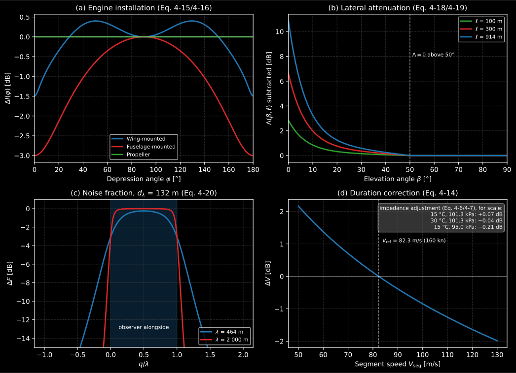
The lateral attenuation is the big term and the only one that can reach double figures: $\Lambda$ is 10.86 dB at grazing incidence and identically zero above an elevation angle of 50°, while the distance factor $\Gamma (\ell )$ ramps from zero on the ground track to unity at 914 m — so a receiver under the track gets none of it and one 900 m to the side at low elevation gets all of it. The installation term is worth 1.5 dB between a wing and a fuselage mounting at $\phi =0$ and nothing at all for a propeller. The duration correction is $10\lg (V_{\text{ref}}/V_{\text{seg}})$, so a departure flown at 100 m/s loses 0.85 dB of exposure per segment. The noise fraction is always negative and vanishes only for an infinite segment. The impedance adjustment is +0.07 dB at the standard atmosphere and rarely leaves a few tenths.

Show the code for this figure

import matplotlib.pyplot as plt
import numpy as np
from phonometry import aircraft

fig, ((ax_i, ax_l), (ax_f, ax_v)) = plt.subplots(2, 2, figsize=(11, 8))
phi = np.linspace(0.0, 180.0, 361)
for mounting in ("wing", "fuselage", "propeller"):
    ax_i.plot(phi, [aircraft.engine_installation_correction(p, mounting)
                    for p in phi], label=mounting)
beta = np.linspace(0.0, 90.0, 361)
for ell in (100.0, 300.0, 914.0):
    ax_l.plot(beta, [aircraft.lateral_attenuation(b, ell) for b in beta],
              label=f"l = {ell:.0f} m")
# The scaled distance of Eq. 4-20 for this NPD table at dp = 526 m.
powers, distances = [8000.0, 12000.0], [60.0, 240.0, 960.0, 3840.0]
sel = [[98.0, 86.0, 74.0, 62.0], [104.0, 92.0, 80.0, 68.0]]
lmax = [[94.0, 82.0, 70.0, 58.0], [100.0, 88.0, 76.0, 64.0]]
base = float(aircraft.npd_level(powers, distances, sel, 12000.0, 526.0)[0])
peak = float(aircraft.npd_level(powers, distances, lmax, 12000.0, 526.0)[0])
d_lambda = (2 / np.pi) * 82.3 * 10 ** ((base - peak) / 10)
frac = np.linspace(-1.0, 2.0, 601)
for length in (464.0, 2000.0):
    ax_f.plot(frac, [aircraft.noise_fraction(f * length, length, d_lambda)
                     for f in frac], label=f"segment {length:.0f} m")
speeds = np.linspace(50.0, 130.0, 401)
ax_v.plot(speeds, [aircraft.duration_correction(82.31104, s) for s in speeds])
for ax in (ax_i, ax_l, ax_f, ax_v):
    ax.grid(True, alpha=0.3)
for ax in (ax_i, ax_l, ax_f):
    ax.legend(fontsize=8)
plt.show()

A single event, segment by segment

event_level does the assembly. Put one receiver 3 km down the track, 500 m to the side of a departure and 1.2 m above the ground, and ask for its sound exposure level:

import numpy as np
from phonometry import aircraft

powers = [8000.0, 12000.0]
distances = [60.0, 120.0, 240.0, 480.0, 960.0, 1920.0, 3840.0, 7680.0]
sel = [[98.0, 92.0, 86.0, 80.0, 74.0, 68.0, 62.0, 56.0],
       [104.0, 98.0, 92.0, 86.0, 80.0, 74.0, 68.0, 62.0]]
lmax = [[94.0, 88.0, 82.0, 76.0, 70.0, 64.0, 58.0, 52.0],
        [100.0, 94.0, 88.0, 82.0, 76.0, 70.0, 64.0, 58.0]]

xs = np.linspace(0.0, 18000.0, 40)                  # ground roll, then a climb
z = np.clip((xs - 1500.0) * 0.11, 0.0, 2500.0)
power = np.where(xs < 3000.0, 12000.0, 10000.0)
path = np.column_stack([xs, np.zeros_like(xs), z, power, np.full_like(xs, 82.3)])
ground_roll = xs[:-1] < 1500.0                      # one entry per segment

flyover = aircraft.event_level(
    path, [3000.0, 500.0, 1.2], powers, distances, sel, lmax,
    segments=aircraft.FlightSegmentState(ground_roll=ground_roll))
seg = flyover.segment_levels
top = int(np.argmax(seg))
print(round(float(flyover.level), 1))               # 82.3 dB: the event SEL
print(top, round(float(seg[top]), 1))               # 6 82.1: the nearest segment
flyover.plot()   # per-segment contributions (needs matplotlib)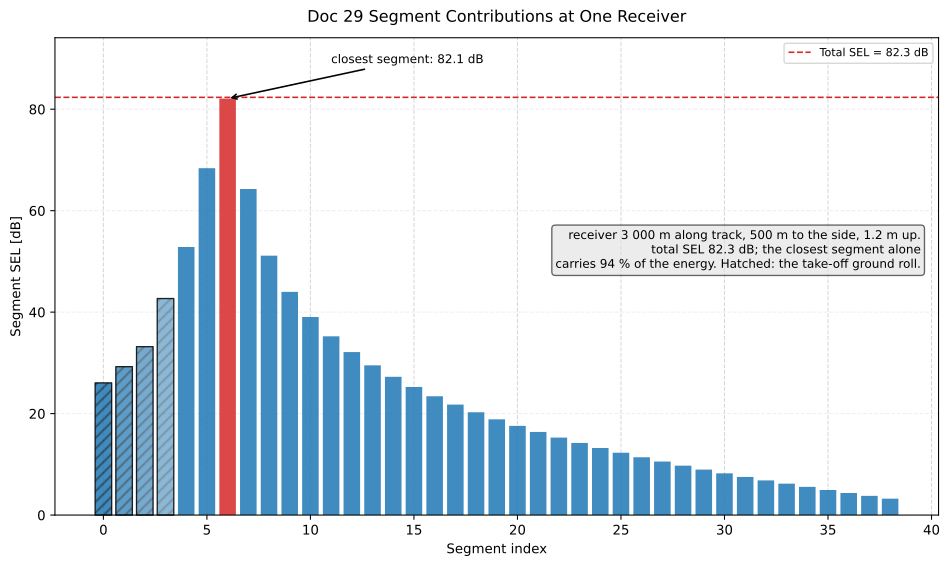

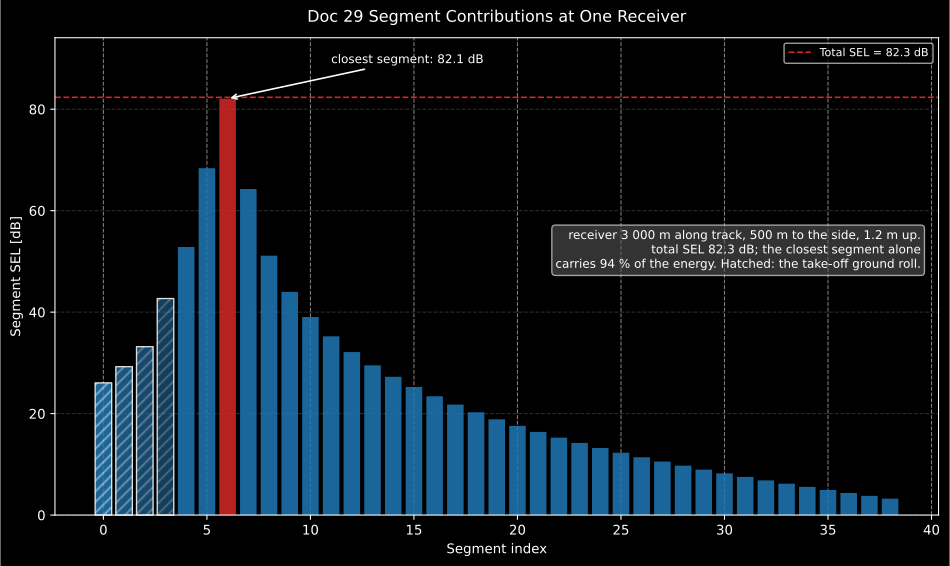
Thirty-nine segments, and one of them is the answer: segment 6 contributes 82.1 dB against a total of 82.3 dB, which is 94 % of the energy. That is what the noise fraction does — the contribution collapses within a couple of segments of the closest point of approach — and it is why a contour is only ever as good as the flight path near each receiver. The ground-roll segments are hatched: they are 40 dB down here, but move the receiver behind the runway and the start-of-roll term brings them back.

Show the code for this figure

import matplotlib.pyplot as plt

ax = flyover.plot()
for i, patch in enumerate(ax.patches[:len(seg)]):
    if ground_roll[i]:
        patch.set_hatch("///")
ax.set_ylim(0.0, float(max(seg)) + 12.0)
plt.show()

The 82.1 dB of that segment is the table plus the five corrections, and nothing else:

s1, s2 = path[top, :3], path[top + 1, :3]
observer = np.array([3000.0, 500.0, 1.2])
u = (s2 - s1) / np.linalg.norm(s2 - s1)
length = float(np.linalg.norm(s2 - s1))               # 464 m of segment
q = float((observer - s1) @ u)                        # 214 m along it
dp = float(np.linalg.norm(observer - (s1 + q * u)))   # 526 m, minimum slant range
beta = float(np.degrees(np.arccos(500.0 / dp)))       # 18.0 deg (§4.5.5)
p_seg = float(np.sqrt(power[top] ** 2
                      + (q / length) * (power[top + 1] ** 2 - power[top] ** 2)))
base = float(aircraft.npd_level(powers, distances, sel, p_seg, dp)[0])
peak = float(aircraft.npd_level(powers, distances, lmax, p_seg, dp)[0])
d_lambda = (2 / np.pi) * 82.3 * 10 ** ((base - peak) / 10)   # Eq. 4-20
terms = {
    "impedance": aircraft.impedance_adjustment(),
    "duration": aircraft.duration_correction(82.3, 82.3),
    "installation": aircraft.engine_installation_correction(beta),
    "lateral": -aircraft.lateral_attenuation(beta, 500.0),
    "noise fraction": aircraft.noise_fraction(q, length, d_lambda),
}
print(round(base, 2), {k: round(v, 2) for k, v in terms.items()})
# 83.89 {'impedance': 0.07, 'duration': 0.0, 'installation': -0.43,
#        'lateral': -1.2, 'noise fraction': -0.25}
print(round(base + sum(terms.values()), 2))           # 82.08, the bar above

The duration correction is exactly zero because the path was flown at the reference speed; the lateral attenuation is only 1.2 dB because the segment is still 18° above the horizon at this receiver; at the same 500 m offset but with the aeroplane on the runway, at grazing incidence, it would be 8.8 dB. noise_contour repeats this calculation at every point of a ground grid, so a contour is worth exactly what this single number is worth.

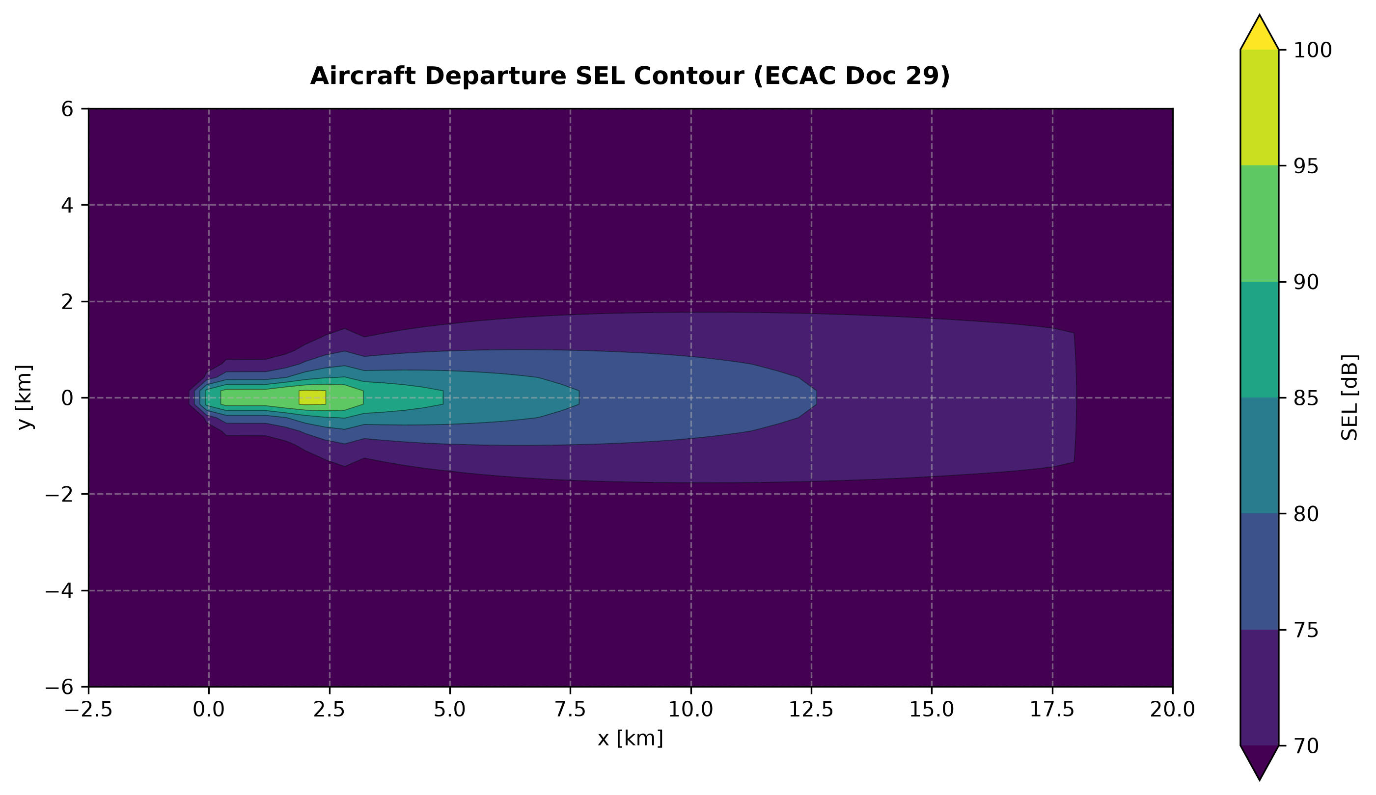
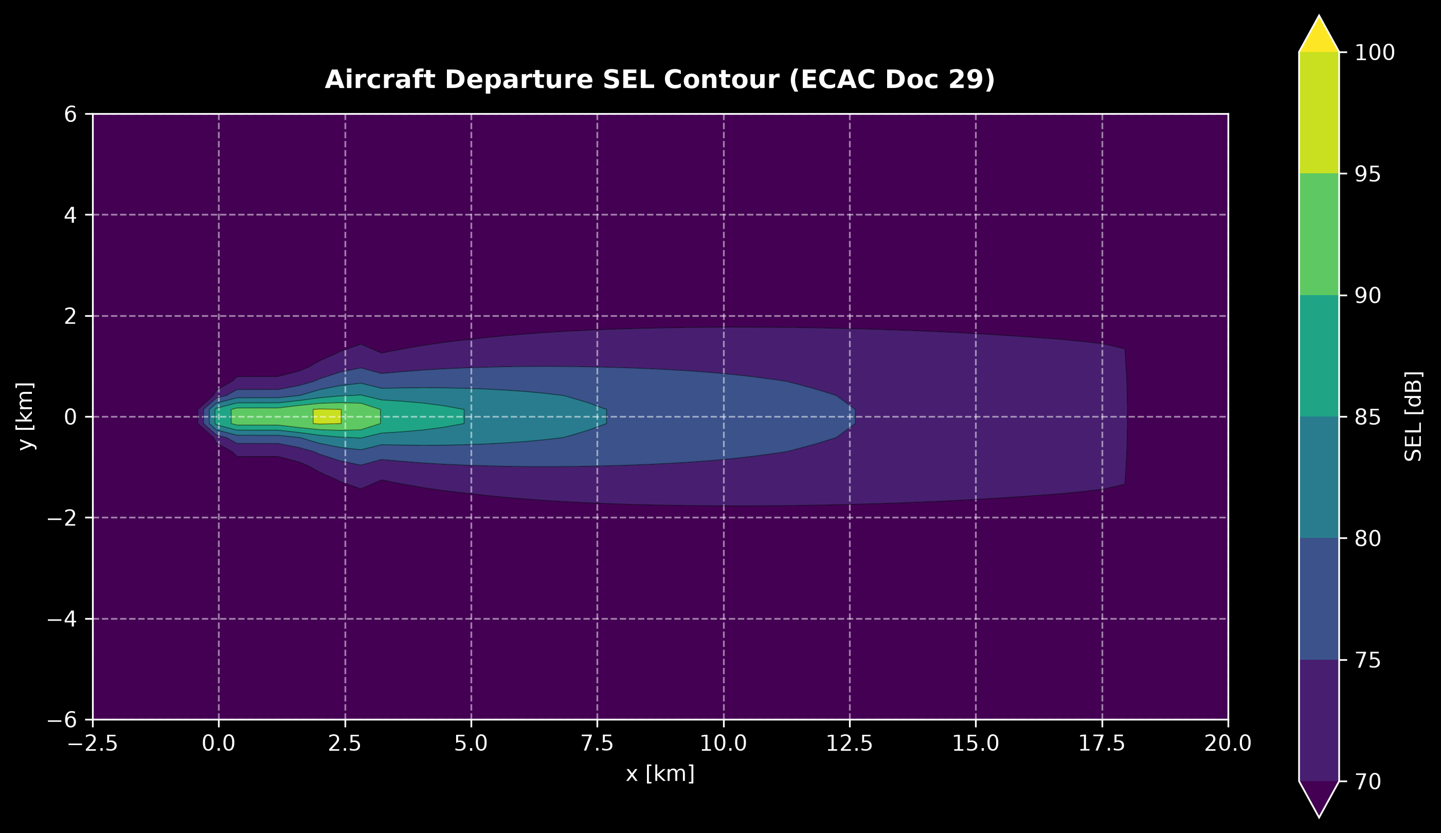
The footprint stretches along the track because every segment contributes to every receiver, and it is widest where the aeroplane is lowest and its slant distances shortest. The sideline levels fall faster than the inverse-square law alone, because lateral attenuation switches on as the elevation angle drops below 50°, and the lobe behind the runway threshold is the start-of-roll directivity of the jet exhaust, which is why the contour does not close symmetrically at the runway end. The outermost contours are the least trustworthy: they are set by the segments at the greatest slant distance, where the NPD table is being extrapolated. This is one movement, not a study — a planning contour accumulates many such events into an $L_{den}$-style index, which is this page’s “Not covered”.

Show the code for this figure

import matplotlib.pyplot as plt
import numpy as np
from phonometry import aircraft

# NPD tables (SEL and LAmax) for one aircraft, two power settings.
powers = [8000.0, 12000.0]
distances = [60.0, 120.0, 240.0, 480.0, 960.0, 1920.0, 3840.0, 7680.0]
sel = [[98.0, 92.0, 86.0, 80.0, 74.0, 68.0, 62.0, 56.0],
       [104.0, 98.0, 92.0, 86.0, 80.0, 74.0, 68.0, 62.0]]
lmax = [[94.0, 88.0, 82.0, 76.0, 70.0, 64.0, 58.0, 52.0],
        [100.0, 94.0, 88.0, 82.0, 76.0, 70.0, 64.0, 58.0]]

# Departure: ground roll along +x, then a steady climb.
xs = np.linspace(0.0, 18000.0, 40)
z = np.clip((xs - 1500.0) * 0.11, 0.0, 2500.0)
power = np.where(xs < 3000.0, 12000.0, 10000.0)
path = np.column_stack([xs, np.zeros_like(xs), z, power, np.full_like(xs, 82.3)])
ground_roll = xs[:-1] < 1500.0   # takeoff roll: segments still on the runway

segments = aircraft.FlightSegmentState(ground_roll=ground_roll)
contour = aircraft.noise_contour(path, powers, distances, sel, lmax,
                                 segments=segments,
                                 x=np.linspace(-2500.0, 20000.0, 56),
                                 y=np.linspace(-6000.0, 6000.0, 44))
contour.plot()   # single-event SEL footprint (needs matplotlib)
plt.show()

The mechanism behind these ground corrections is two-path interference: the direct wave and its ground reflection. Below, a 400 Hz source 1.5 m above a rigid plane forms the lobe pattern, with the image source ghosted below the ground and a receiver sitting in an interference dip.

A 2D FDTD simulation of a 400 Hz point source 1.5 metres above rigid ground. The direct and ground-reflected wavefronts interfere and a lobe pattern forms, the ghosted image source below the ground explains the geometry, and the level sampled on an 8 metre arc converges to the two-path image-source model with its predicted nulls.

Download the animation (WebM)

A 2D FDTD simulation of a 400 Hz point source 1.5 metres above rigid ground. The direct and ground-reflected wavefronts interfere and a lobe pattern forms, the ghosted image source below the ground explains the geometry, and the level sampled on an 8 metre arc converges to the two-path image-source model with its predicted nulls.

Download the animation (WebM)

The start-of-roll directivity is the lobed rearward radiation of jet-exhaust noise: strongest near an azimuth $\psi \approx 120°$ from the nose, falling off abeam ($\psi =90°$) and directly behind ($\psi =180°$).

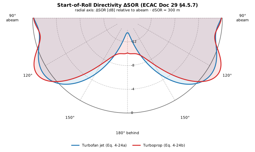
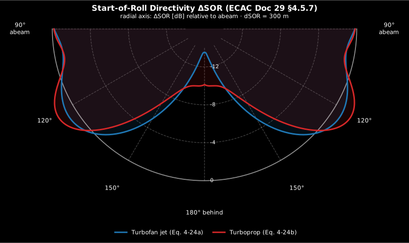
The lobe is narrow and the penalty behind it is large. At 300 m the jet peaks at +0.99 dB at $\psi$ = 123° and the turboprop at +1.96 dB at 121°, both within 0.2 dB of abeam at 90°; by 180°, straight behind the aircraft, they are down to −13.5 and −10.1 dB. A receiver placed a few degrees off the lobe therefore sees a completely different start-of-roll contribution, which is why ${\Delta }_{SOR}$ is applied per segment and per receiver rather than as a single correction to the event.

Show the code for this figure

import matplotlib.pyplot as plt
import numpy as np
from phonometry import aircraft

az = np.linspace(90.0, 270.0, 361)              # rearward semicircle
psi = np.where(az <= 180.0, az, 360.0 - az)     # ΔSOR is left/right symmetric
jet = [aircraft.start_of_roll_directivity(p, 300.0, "jet") for p in psi]
prop = [aircraft.start_of_roll_directivity(p, 300.0, "turboprop") for p in psi]

ax = plt.subplot(projection="polar")
ax.set_theta_zero_location("N")                 # nose up, azimuth clockwise
ax.set_theta_direction(-1)
ax.plot(np.radians(az), jet, label="Turbofan jet")
ax.plot(np.radians(az), prop, label="Turboprop")
ax.set_rlim(-16.0, 0.0)                         # radial axis: dB re abeam
ax.legend(loc="lower center")
plt.show()

import numpy as np
from phonometry import aircraft

powers = [8000.0, 12000.0]; distances = [60.0, 240.0, 960.0, 3840.0]
sel = [[98.0, 86.0, 74.0, 62.0], [104.0, 92.0, 80.0, 68.0]]
lmax = [[94.0, 82.0, 70.0, 58.0], [100.0, 88.0, 76.0, 64.0]]
xs = np.linspace(0.0, 18000.0, 40)
path = np.column_stack([xs, np.zeros_like(xs), np.clip((xs-1500)*0.11, 0, 2500),
                        np.where(xs < 3000, 12000.0, 10000.0), np.full_like(xs, 82.3)])
ground_roll = xs[:-1] < 1500.0   # takeoff roll: segments still on the runway
aircraft.noise_contour(path, powers, distances, sel, lmax,
                 segments=aircraft.FlightSegmentState(ground_roll=ground_roll),
                 x=np.linspace(-2500, 20000, 60), y=np.linspace(-6000, 6000, 48)).plot()

Validated against the ECAC Doc 29 5th ed. Vol 3 Part 1 reference workbook: the segment geometry, lateral attenuation, engine installation, noise fraction and the start-of-roll directivity (turbofan and turboprop) reproduce the reference values to $<0.01\text{dB}$, and the segment energy sum matches the reference SEL.

Four more pieces of the method are in place. The landing rollout is the landing_roll mask of the FlightSegmentState: ahead of it the noise fraction takes its reduced form (Eq. 4-21b) and the nearest-end geometry applies, with no directivity term, because Doc 29 assumes a semicircular horizontal directivity there. The per-segment bank angle is its bank, positive with the starboard wing up, and it selects the branch of $\phi =\beta \pm \epsilon$ by which side of the track the receiver is on (§4.5.2). Behind a take-off ground roll the §4.5.5 nearest-end lateral geometry replaces the equivalent-level-path one, which is the same switch that makes the NPD lookup use $d_s$ there. And a runway segment takes the Eq. 4-13b average of its end speeds rather than the quadratic interpolation an airborne segment uses, while every NPD lookup is floored at the recommended 30 m. Seven branch-covering receptor events of the reference workbook are reproduced end-to-end in the test suite.

What this guide covers

• Covered

  The ECAC Doc 29 single-event airport-noise chain: the NPD interpolation of npd_level/npd_curve (Eqs. 4-3, 4-4), the per-segment corrections impedance_adjustment, lateral_attenuation (SAE AIR 5662 soft ground), engine_installation_correction, duration_correction, noise_fraction and start_of_roll_directivity, their assembly into SEL/$L_{Amax}$ by event_level and the ground-grid noise_contour, including the landing rollout, per-segment bank angle and the nearest-end lateral geometry. Validated to under 0.01 dB against the Doc 29 5th ed. Vol. 3 Part 1 reference workbook.

• Not covered

  The chain builds single-event contours only: it does not assemble the cumulative multi-event indices (an $L_{den}$-style sum over a full flight schedule) that a complete Doc 29 noise-contour study needs on top of these single-event levels. NPD tables themselves are an input, not a prediction: the library interpolates the tables supplied for an aircraft type, it does not synthesise them from engine data. The EASA/EUROCONTROL ANP database of measured tables for real types does ship with phonometry and is read by The ANP fleet database, which wires it straight into the functions of this page. Converting NPD data to a site outside the §2.5 envelope (the Appendix D recalculation) is not implemented, and neither is the acoustically hard ground that SAE AIR 5662 excludes: the lateral attenuation, and with it the whole single-event chain, assumes soft grassy ground.

See also

• Aircraft noise: Effective Perceived Noise Level: the ICAO Annex 16 certification metric behind the aircraft data.
• The ANP fleet database: the shipped NPD tables and default trajectories for real aircraft types, which run this chain without a hand-written table.
• Rotorcraft noise: the hemisphere method: the ECAC Doc 32 contour method, where a noise hemisphere plays the role the NPD table plays here. Mind the symbols on the way across: Doc 32 uses $\phi$ for the hemisphere azimuth and writes the bank angle $\Phi$, where Doc 29 uses $\phi$ for the depression angle and $\epsilon$ for the bank. Each is its own standard’s notation.
• Outdoor sound propagation: the ISO 9613-2 attenuation terms and the ground effect the lateral attenuation condenses into one curve.
• Environmental Levels: the $L_{den}$-style long-term indices that a full airport study accumulates from single events.
• API reference: aircraft.airport_noise.

References

• European Civil Aviation Conference. (2016). Report on standard method of computing noise contours around civil airports, Volume 2: Technical guide (ECAC.CEAC Doc 29, 4th ed.). The NPD event-level interpolation (section 4.2) and the single-event segment calculation (impedance adjustment, duration, engine installation, lateral attenuation, noise fraction, start-of-roll directivity, summation) of this guide, up to the ground-grid noise contours. The linked PDF is the free download; the volumes are catalogued on the ECAC documents page (https://www.ecac-ceac.org/documents/ecac-documents-and-international-agreements).
• European Civil Aviation Conference. (2026). Report on standard method of computing noise contours around civil airports, Volume 3: Reference cases and verification framework (ECAC.CEAC Doc 29, 5th ed.). The Part 1 reference workbook the single-event chain is validated against. The linked PDF is the free download; the volumes are catalogued on the ECAC documents page (https://www.ecac-ceac.org/documents/ecac-documents-and-international-agreements).
• SAE International. (2006). Method for predicting lateral attenuation of airplane noise (SAE AIR 5662). The soft-ground lateral-attenuation model that Doc 29 adopts (section 4.5.4) in the single-event contour section.