Rotorcraft noise: the hemisphere method

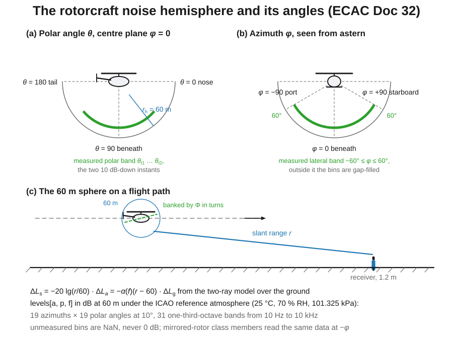
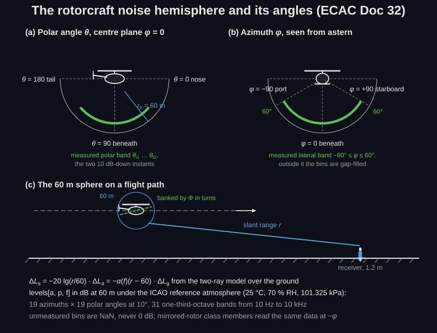
Helicopter noise is strongly directive, so the ECAC Doc 32 method describes the source with a noise hemisphere: one-third-octave-band sound pressure levels on a spherical grid of azimuth $\phi$ and polar angle $\theta$, defined at a fixed 60 m reference distance under ICAO reference atmospheric conditions. Placing that source at a receiver adds the propagation adjustment $\Delta L_p=\Delta L_s+\Delta L_a+\Delta L_g$.

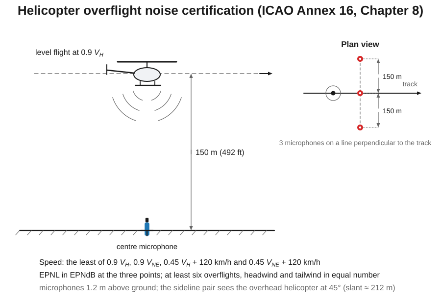
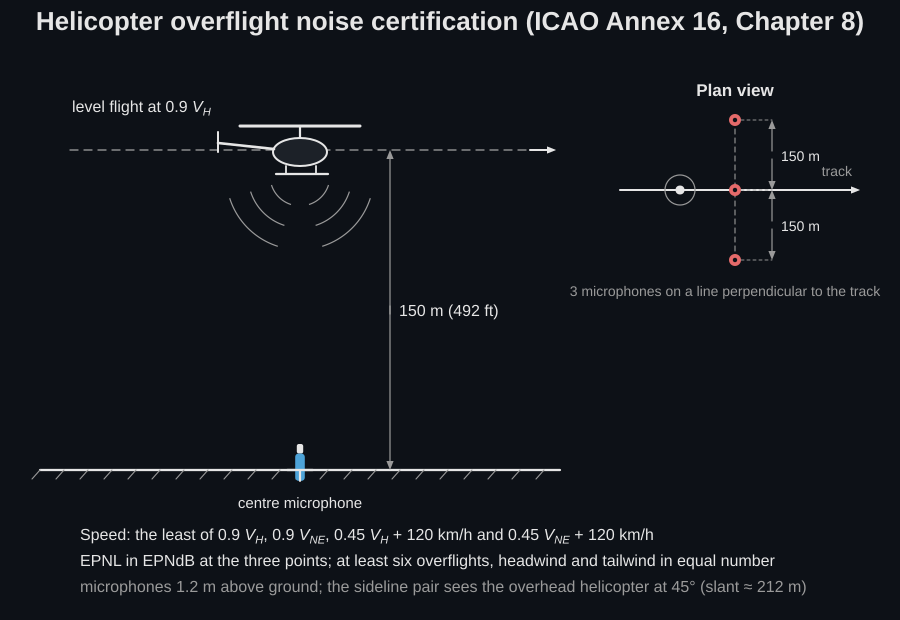
The EPNL this page computes is the same quantity fixed-wing certification asks for; only the source description differs. ICAO Annex 16 Chapter 8 flies the helicopter level at 150 m over a centre microphone, with two more 150 m to each side.

Where a hemisphere comes from

The library implements the method, not the data: no hemisphere database ships with phonometry, and there is no NORAH file reader, so the arrays below have to be assembled by the reader. There are two places they come from. One is a flight-test campaign: the rotorcraft is flown over a ground microphone array, each emission direction’s spectrum is de-propagated back to a 60 m reference sphere under ICAO noise-certification reference conditions (101 325 Pa, 298.15 K, 70 % relative humidity), and the measurement follows the Annex 16 Vol. I practice Doc 32 §4.2 points at. The other is the NORAH2 reference database, which covers eleven rotorcraft types.

A usable hemisphere carries more than levels. The NORAH file format (Doc 32 Appendix A) records the reference distance POLDIST, whether atmospheric absorption is included, the no-value indicator, the hemisphere’s own atmosphere (TAMB, RELHUM, PAMB), and then the conditions the data was acquired at: the measurement temperature, humidity and pressure at 10 m, the rotor speed, the indicated airspeed, the path angle, the pitch and roll attitudes and the wind components. The airspeed and the path angle are not metadata: they are the key the flight-condition interpolation below looks the hemisphere up by, so a hemisphere without them cannot be placed in a database.

What a ground array can see is limited, and that is why real hemispheres arrive with holes. Doc 32 requires coverage of at least $-60°\le \phi \le 60°$ and the polar angles between the two 10 dB-down instants; measuring wider lateral angles, or polar angles approaching 0° and 180°, needs a more elaborate setup. The gap-filling of Eq. 6/7 is the direct consequence of that limit, not an implementation detail — outside the measured patch the level is the nearest filled bin’s, and the energetic average of them where several are equally near.

The condition matrix a database should span is fixed by Doc 32 §4.1: hemispheres at descent angles at intervals of at least 3° and four different airspeeds, to cover the descent region where blade-vortex interaction lives; climb angles at the best rate-of-climb speed $V_y$ or a typical take-off speed, including the maximum climb angle stated in the flight manual; and level flight at 0.9 $V_H$ with $+10$ kt (or $V_H$, whichever is smaller), $-15$ kt and $-30$ kt increments. Outside the hull those conditions span, the interpolation degrades to nearest-neighbour, silently.

When a class has no hemisphere at all, Doc 32 §3.2 gives the substitution rule: group the type temporarily with a class that does have one, choosing a class whose certification noise levels are lower than or within the range of the target’s; where certification levels are unavailable or several classes qualify, weight becomes the governing parameter and the best-matching class below the type’s weight is taken, with the level offset $\Delta \mathrm{EPNL}$ set to zero so the estimate stays conservative. Within a class, the offset is the difference in registered certification levels — take-off, overflight and approach levels correcting the climb, level and descent conditions respectively — and it enters here as level_offset.

The noise hemisphere

A RotorcraftHemisphere holds the band levels on the azimuth/polar grid.

Field	Shape	Units and convention
frequencies	(F,)	one-third-octave band centres in Hz; the NORAH format carries 31 bands from 10 Hz to 10 kHz
azimuth $\phi$	(A,)	degrees about the nose axis: $0$ straight down, $+90$ starboard, $-90$ port; 19 values at 10°
polar $\theta$	(P,)	degrees from the nose: $0$ forward, $90$ across the aircraft, $180$ rearward; 19 values at 10°
levels	(A, P, F)	band sound pressure levels in dB at the reference distance; NaN in bins the measurement did not cover
distance	scalar	reference distance in metres, 60 by default

The two angles are the spherical coordinates of Doc 32 Eq. 3, $x=r\cos \theta$, $y=r\sin \theta \sin \phi$, $z=r\sin \theta \cos \phi$ in body axes with $z$ down, so $\theta$ is measured from the nose and $\phi$ rotates about the nose axis starting from straight down. hemisphere_source_level(h, azimuth_deg, polar_deg) takes the angles in that order and returns one level per band: hemisphere_source_level(h, 0.0, 90.0) is the level radiated vertically downwards, which is what a microphone directly under a level flyover hears, while a receiver 500 m to the side of the same overflight at 150 m is addressed at roughly $(\phi ,\theta )=(73°,90°)$. Getting the sign of $\phi$ backwards mirrors the aircraft; treating $\theta$ as an angle from the vertical transposes the array and gives a plausible but wrong directivity. NaN and 0 dB are not interchangeable: unmeasured bins must be NaN, because they are gap-filled from the angularly nearest filled bin before the bilinear lookup, and a stored 0 dB would be taken as data. h.mirrored() implements the rotor-sense relation of Eq. 2 by reversing the azimuth sign.

hemisphere_source_level reads the level at an arbitrary emission direction: the grid is first gap-filled from the angularly-nearest filled bins (Eq. 14/15, cached), then the lookup is bilinear in the energy domain over the four neighbouring bins (Eq. 13), so partially-measured cells stay continuous with their measured corners.

from phonometry import aircraft

h = aircraft.RotorcraftHemisphere(frequencies=freqs, azimuth=phi, polar=theta, levels=levels)
lv = aircraft.hemisphere_source_level(h, 0.0, 90.0)   # straight down, per band, at 60 m
h.plot()                                          # fore-aft directivity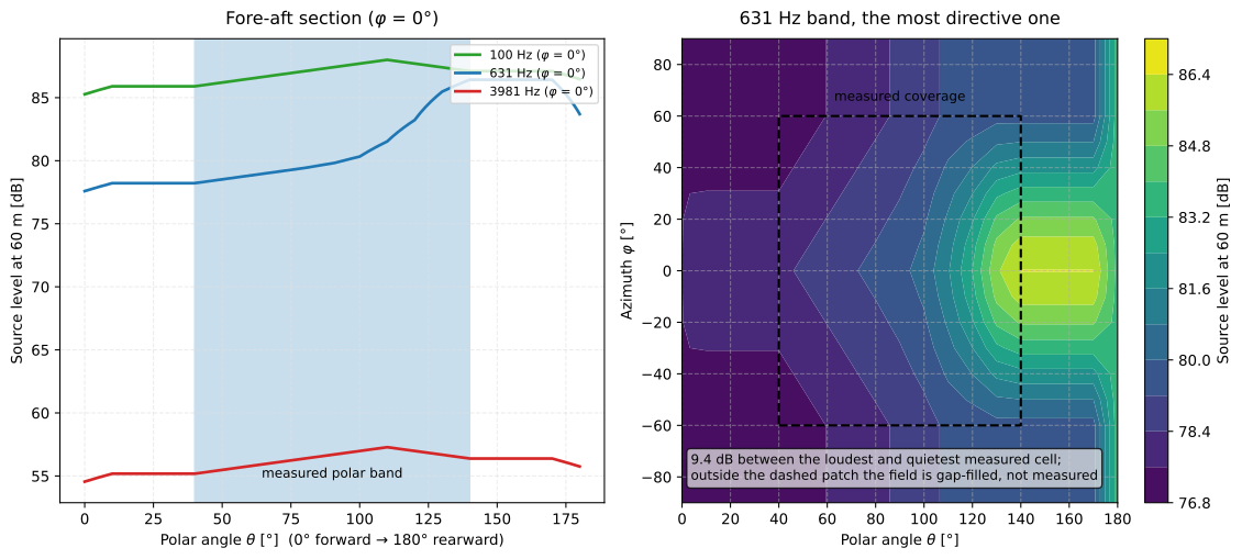

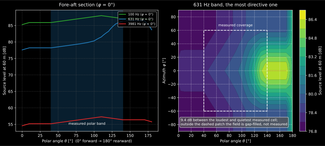
Why the method needs a hemisphere at all: in the most directive band, 9.4 dB separate the loudest measured direction from the quietest, and the lobe sits at $\theta \approx 140°$, well aft of the vertical. The three sections on the left show that the directivity is frequency-dependent — the low band is nearly flat, the mid band carries the lobe, the high band is quiet everywhere — so a single source level cannot stand in for it. Note also what the curves do outside the shaded band: they go flat. That is the gap-filling, not measurement.

Show the code for this figure

import matplotlib.pyplot as plt
import numpy as np
from phonometry import aircraft

# A synthetic hemisphere on the Doc 32 grid: 31 bands, 19 x 19 angles, with a
# mid-frequency lobe behind abeam and the cells a ground array cannot see left
# as NaN.
freqs = 1000.0 * 10.0 ** (np.arange(-20, 11) / 10.0)
az, po = np.arange(-90.0, 91.0, 10.0), np.arange(0.0, 181.0, 10.0)
spectrum = 88.0 - 12.0 * np.log10(freqs / 100.0) ** 2
band = np.exp(-((np.log10(freqs) - np.log10(630.0)) ** 2) / 0.08)
levels = (spectrum[None, None, :]
          - 0.030 * np.abs(po - 110.0)[None, :, None]
          - 0.020 * np.abs(az)[:, None, None]
          + 7.0 * np.exp(-((po - 140.0) ** 2) / (2 * 16.0 ** 2))[None, :, None]
          * np.exp(-(az ** 2) / (2 * 34.0 ** 2))[:, None, None]
          * band[None, None, :])
unseen = (np.abs(az)[:, None] > 60.0) | (po[None, :] < 40.0) | (po[None, :] > 140.0)
h = aircraft.RotorcraftHemisphere(freqs, az, po, np.where(unseen[:, :, None],
                                                          np.nan, levels))

fig, (ax, ax2) = plt.subplots(1, 2, figsize=(12, 5.4))
for f in (100.0, 630.0, 4000.0):
    h.plot(ax=ax, band=f)
ax.axvspan(40.0, 140.0, color="0.85", zorder=0)
idx = int(np.nanargmax(np.nanmax(levels, axis=(0, 1)) - np.nanmin(levels, axis=(0, 1))))
filled = np.array([[aircraft.hemisphere_source_level(h, a, p)[idx] for p in po]
                   for a in az])
cs = ax2.contourf(po, az, filled, levels=12)
ax2.plot([40, 140, 140, 40, 40], [-60, -60, 60, 60, -60], "k--")
fig.colorbar(cs, ax=ax2, label="Source level at 60 m [dB]")
plt.show()

Propagation adjustments

The 60 m hemisphere level is carried to the receiver by three adjustments (§A.4): spherical_spreading_adjustment ($\Delta L_s=-20{\log }_{10}(r/60)$, Eq. 24), atmospheric_adjustment ($\Delta L_a=-\alpha (f)(r-60)$ with the ISO 9613-1 coefficient, Eq. 26/27), and ground_effect_adjustment (direct/reflected interference over an impedance plane, Chien-Soroka Eq. 28-35, with the Delany-Bazley impedance and the CNOSSOS flow-resistivity classes "A"-"H").

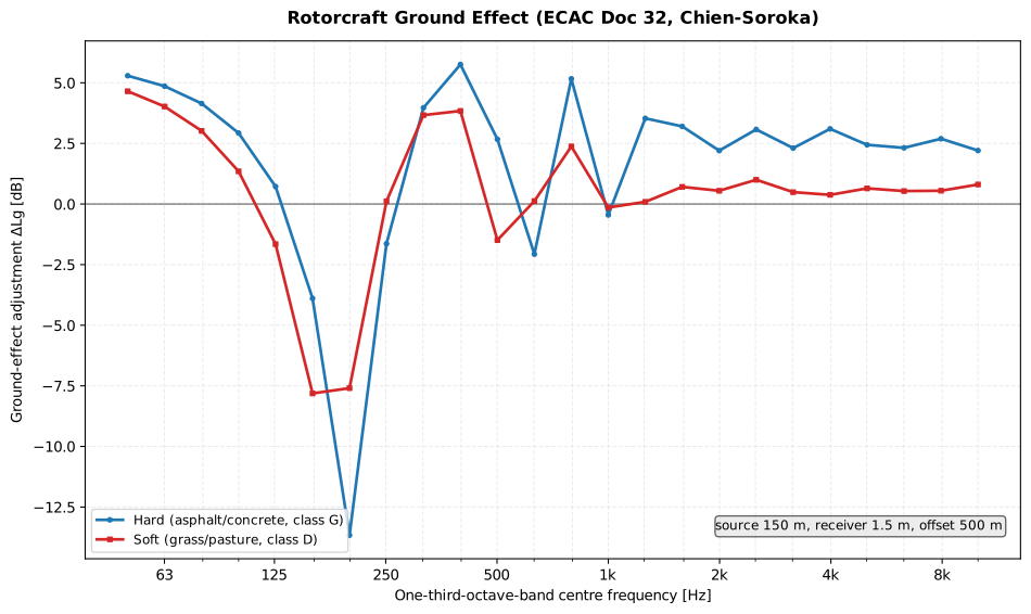
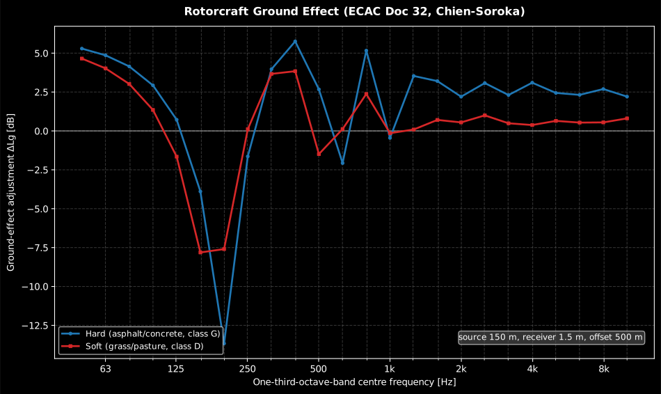
One geometry, two ground classes, and the hard surface is the more extreme in both directions: it reinforces more at low frequency (+5.3 dB against +4.7 dB at 50 Hz), cancels far more completely at the first minimum (−13.7 dB against −7.8 dB) and is still oscillating around +2.4 dB at 5 kHz where the soft curve has settled towards an incoherent sum near +0.6 dB. The three regions are read below the code.

Show the code for this figure

import matplotlib.pyplot as plt
import numpy as np
from phonometry import aircraft

freqs = 1000.0 * 10.0 ** (np.arange(-13, 11) / 10.0)   # 50 Hz-10 kHz thirds
hs, hr, dp = 150.0, 1.5, 500.0                          # overflight geometry
grass = aircraft.ground_effect_adjustment(freqs, hs, hr, dp, flow_resistivity="D")
asphalt = aircraft.ground_effect_adjustment(freqs, hs, hr, dp, flow_resistivity="G")

fig, ax = plt.subplots()
ax.axhline(0.0, color="0.5", linewidth=1.0)
ax.semilogx(freqs, asphalt, marker="o", markersize=3,
            label="Hard (asphalt/concrete, class G)")
ax.semilogx(freqs, grass, marker="s", markersize=3,
            label="Soft (grass/pasture, class D)")
ax.set(xlabel="One-third-octave-band centre frequency [Hz]",
       ylabel="Ground-effect adjustment ΔLg [dB]",
       title="Rotorcraft ground effect (ECAC Doc 32, Chien-Soroka)")
ax.grid(True, which="both", alpha=0.3)
ax.legend()
plt.show()

import numpy as np
from phonometry import aircraft

freqs = 1000.0 * 10.0 ** (np.arange(-13, 11) / 10.0)   # 50 Hz-10 kHz thirds
r = 500.0
received = (lv
            + aircraft.spherical_spreading_adjustment(r)
            + aircraft.atmospheric_adjustment(freqs, r)
            + aircraft.ground_effect_adjustment(freqs, 150.0, 1.5, 500.0, flow_resistivity="D"))

The standard database is recorded at 60 m, the default. If a hemisphere uses a different polar distance (h.distance, e.g. 70 m hover rings), pass it to both distance-dependent adjustments as reference_distance=h.distance.

Read the ground curve as three regions. At low frequency the direct ray and its ground reflection arrive almost in phase, so the level approaches 6 dB above free field — 5.3 dB at 50 Hz over hard ground in the figure, rising to 5.8 dB. The first cancellation sits where the path difference is half a wavelength, which for this geometry — the source 150 m up, the microphone 1.5 m and 500 m of horizontal offset — falls at 200 Hz and is 13.7 dB deep; it marches upward as the aircraft passes overhead, so the adjustment is a moving comb rather than a fixed spectrum shape. Over grass the finite impedance rotates the phase of the reflected wave and absorbs part of it, so the reinforcement is a little smaller (4.7 dB at 50 Hz) and, more importantly, the cancellation is far less complete: the first minimum is 7.8 dB rather than 13.7 dB. At high frequency the two paths decorrelate towards an incoherent sum, which is where the soft curve settles near 0.6 dB while the hard one is still ringing at 2.4 dB at 5 kHz. All of it is coherent by construction, so a level averaged over a whole event shows far less structure than any single frozen spectrum here.

Three site parameters decide the ground term, and the default is not the one a grass site wants:

Field	Default	What to set it to
receiver_height	1.2 m	the Annex 16 microphone height; the figure above uses 1.5 m to make the dip visible
ground_elevation	0.0 m	per receiver on uneven sites, or one value per grid point
flow_resistivity	"G"	hard ground. A grass or pasture site must pass "C" or "D"

The letters are the CNOSSOS-EU classes of Doc 32 Table 3, in Pa·s/m²: "A" very soft (snow, moss) at 12.5·10³, "B" soft forest floor at 31.5·10³, "C" uncompacted loose ground — turf, grass, loose soil — at 80·10³, "D" normal uncompacted ground such as pasture at 200·10³, "E" compacted field and gravel at 500·10³, "F" compacted dense ground such as a gravel road or car park at 2·10⁶, "G" hard surfaces, most normal asphalt and concrete, at 20·10⁶, and "H" very hard and dense surfaces including water at 200·10⁶. A numeric σ in Pa·s/m² is accepted in place of a letter, and so is an array with one value per grid point.

The atmosphere is silent in the same way. The hemisphere is defined under the ICAO reference conditions and already contains the absorption of the first 60 m, which is why only the excess path is corrected; the coefficient for that excess path defaults to those same reference conditions (25 °C, 70 % RH, 101.325 kPa) unless a RotorcraftAtmosphere is passed. The difference is largest exactly where a helicopter spectrum still carries energy — the upper third-octave bands over long slant paths — so a cold, dry or high-altitude site needs the argument. atmospheric_method selects "iso9613" (the default) or "sae"; the two agree to about 0.05 dB below 3.15 kHz.

Flight conditions: interpolating between hemispheres

A database records one hemisphere per flight condition (airspeed $V$, path angle $\gamma$). Real conditions rarely coincide with a measured one, so the NORAH2 guidance interpolates (Eq. 3-10): both axes are normalised by their database spans (with the empirical factor $F_{\text{fc}}=2$ on the path angle), a Delaunay triangulation covers the normalised conditions, and a query inside the convex hull blends its enveloping triangle with inverse-distance weights in the energy domain. Outside the hull the nearest condition is adopted unblended, which is also the behaviour ECAC Doc 32, 1st ed. prescribes for its whole envelope (it defines no interpolation yet).

from phonometry import aircraft

speeds = [50.0, 70.0, 60.0]                # one hemisphere per condition
angles = [0.0, 0.0, 10.0]                  # path angles, degrees
weights = aircraft.flight_condition_weights(speeds, angles, 60.0, 2.5)
lv = aircraft.interpolated_source_level(
    [h_50_level, h_70_level, h_60_climb], speeds, angles,
    60.0, 2.5, 0.0, 90.0)                  # blended level per band

The airspeed, not the ground speed, selects the hemisphere; the weights are unit-invariant as long as the query matches the database units. Mirrored-rotor class members substitute h.mirrored() (Eq. 2, $\phi \to -\phi$) and certification-level offsets enter as level_offset.

Two triangulations are in play, and they do not agree. By default the library triangulates the normalised $(V/\Delta V,F_{\text{fc}}\gamma /\Delta \gamma )$ plane, which keeps the two axes comparable for an arbitrary database. The NORAH tables instead ship a triangulation of the raw $(V,\gamma )$ plane, and it must be passed as triangles whenever you are reproducing a NORAH result — because the two disagree about which simplex encloses a query, and therefore about the blend weights.

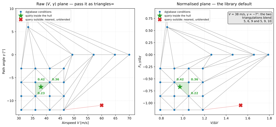
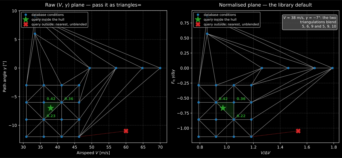
The same query, two triangulations, two different triples of hemispheres blended. The diagonal of the quadrilateral around it flips between the raw and the normalised plane, so the raw triangulation blends conditions 5, 6 and 9 and the normalised one blends 5, 9 and 10. Both are defensible; only one reproduces NORAH. Outside the hull neither blends at all, and the nearest condition is adopted whole — which changes the answer without raising anything, and is the trap worth knowing about.

Show the code for this figure

import matplotlib.pyplot as plt
import numpy as np
from scipy.spatial import Delaunay
from phonometry import aircraft

# A Doc 32 4.1 condition matrix: descent at 3 deg steps and four airspeeds,
# climb at Vy, and level flight at 0.9 VH with the recommended increments.
speeds = list(np.repeat([30.9, 36.0, 41.2, 46.3], 4)) + [33.4, 33.4, 64.8, 70.0, 57.1, 49.4]
angles = list(np.tile([-3.0, -6.0, -9.0, -12.0], 4)) + [6.0, 9.0, 0.0, 0.0, 0.0, 0.0]
v, g = np.asarray(speeds), np.asarray(angles)
raw_tri = Delaunay(np.column_stack([v, g])).simplices

print(aircraft.flight_condition_weights(v, g, 38.0, -7.0))
print(aircraft.flight_condition_weights(v, g, 38.0, -7.0, triangles=raw_tri))
# [(5, 0.42), (9, 0.36), (10, 0.22)]  and  [(5, 0.42), (6, 0.23), (9, 0.36)]

fig, ax = plt.subplots(figsize=(6, 5))
ax.triplot(v, g, raw_tri, color="0.6", lw=0.9)
ax.plot(v, g, "o", ms=5)
ax.plot([38.0], [-7.0], "*", ms=15)
ax.set(xlabel="Airspeed V [m/s]", ylabel="Path angle γ [°]")
plt.show()

Hover, idle and taxi (Table 3)

A hovering or idling helicopter is measured differently from a flyover: on a ring of ground microphones around the stationary aircraft (the CAEP in-ground hover practice the guidance points at), one band spectrum per ring bearing — 0° at the nose, positive to starboard — reduced to the ring’s polar distance, commonly 70 m rather than the flyover database’s 60 m. Guidance §A.3.5 defines four conditions — in-ground hover (HIGE), out-of-ground hover (HOGE), reduced-rpm idle and full-rpm idle — and three approaches in descending priority: measure all four rings; measure the HIGE ring and the other three in the 0° direction only; or measure the HIGE ring alone and apply fixed offsets.

hover_ring_hemisphere extends the ring to a full RotorcraftHemisphere “assuming constant directivity in φ”: each bin $(\phi ,\theta )$ reads the ring at the bearing $\pm \theta$ of its own half — port bins from negative bearings, starboard bins from positive ones, and the $\phi =0$ column under the aircraft takes the energy mean of the $\pm \theta$ ring values — interpolating periodically in the energy domain. The NORAH2 reference implementation reads the same ring by the horizontal bearing of the emission direction instead (constant directivity in elevation): mapping="bearing" reproduces it. The two readings coincide on the hemisphere rim and part by several dB at steep emission angles — directly beneath the hover the constant-φ reading averages port and starboard where the prototype reads the nose bearing.

hover_derived_hemisphere then derives HOGE and the idles from the HIGE hemisphere by a uniform level offset: a measured 0°-direction difference (Approach 2, passed as offset_db), or the published Approach 3 constants — +12 dB for HOGE, −12 dB for reduced-rpm idle and −2.5 dB for full-rpm idle, all from the HIGE disk. A constant spectral shift moves the A-weighted level by exactly that value, which is how Table 3 (stated on $L_A$ levels) extends to band spectra.

import numpy as np
from phonometry import aircraft

# A hover ring with a real campaign's shape: one 31-band third-octave
# spectrum per 30° of bearing, reduced to the 70 m polar distance.
freqs = 1000.0 * 10.0 ** (np.arange(-20, 11) / 10.0)    # 10 Hz-10 kHz thirds
bearings = np.arange(-180.0, 151.0, 30.0)               # the ring closes at ±180°
ring_levels = (86.0 - 10.0 * np.log10(freqs / 160.0) ** 2
               + 3.5 * np.cos(np.radians(bearings))[:, None])
hige = aircraft.hover_ring_hemisphere(freqs, bearings, ring_levels, distance=70.0)
hoge = aircraft.hover_derived_hemisphere(hige, "out_of_ground_hover")   # +12 dB
full_rpm_idle = aircraft.hover_derived_hemisphere(hige, "full_rpm_idle")  # -2.5 dB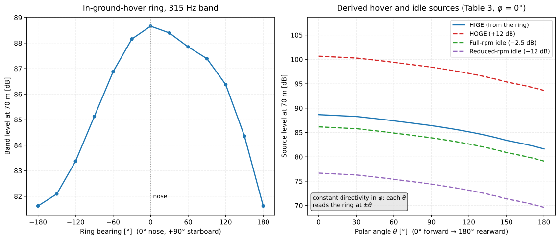

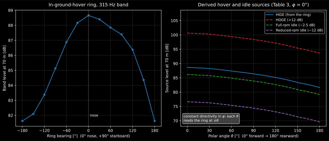
The ring on the left is the only measurement; everything on the right is derived from it. The HIGE section starts at the ring’s nose value and ends at its tail value — that is the constant-φ extension at work — and the other three sources are the same directivity shifted whole: +12 dB up to HOGE, −2.5 dB to full-rpm idle, −12 dB to reduced-rpm idle.

Show the code for this figure

import matplotlib.pyplot as plt
import numpy as np
from phonometry import aircraft

freqs = 1000.0 * 10.0 ** (np.arange(-20, 11) / 10.0)   # 10 Hz-10 kHz thirds
bearings = np.arange(-180.0, 151.0, 30.0)
spectrum = 86.0 - 10.0 * np.log10(freqs / 160.0) ** 2
directivity = (3.5 * np.cos(np.radians(bearings))
               + 3.0 * np.exp(-((bearings - 120.0) ** 2) / (2.0 * 40.0**2)))
ring = spectrum[None, :] + directivity[:, None]
hige = aircraft.hover_ring_hemisphere(freqs, bearings, ring, distance=70.0)

k = int(np.argmin(np.abs(freqs - 315.0)))
theta = np.linspace(0.0, 180.0, 361)
fig, (ax, ax2) = plt.subplots(1, 2, figsize=(12, 5.2))
ax.plot(np.append(bearings, 180.0), np.append(ring[:, k], ring[0, k]),
        marker="o")
ax.set(xlabel="Ring bearing [°]  (0° nose, +90° starboard)",
       ylabel="Band level at 70 m [dB]")
for condition, label in ((None, "HIGE (from the ring)"),
                         ("out_of_ground_hover", "HOGE (+12 dB)"),
                         ("full_rpm_idle", "Full-rpm idle (-2.5 dB)"),
                         ("reduced_rpm_idle", "Reduced-rpm idle (-12 dB)")):
    h = hige if condition is None else aircraft.hover_derived_hemisphere(hige, condition)
    ax2.plot(theta, [aircraft.hemisphere_source_level(h, 0.0, t)[k] for t in theta],
             label=label)
ax2.set(xlabel="Polar angle θ [°]  (0° forward → 180° rearward)",
        ylabel="Source level at 70 m [dB]")
ax2.legend()
plt.show()

The published offsets and the shipped ones

The guidance warns that its constants come from measurements with inverted microphones on ground plates and may not hold for other setups — and the NORAH2 public database actually ships +8/−10/−2 dB in every type’s interpolation file. Pass those as offset_db to reproduce the prototype; the published Table 3 constants are the defaults. The Approach 3 prose also derives full-rpm idle from HOGE where its own table derives it from HIGE, 12 dB apart; the table, backed by the database, is what is implemented. Both divergences are recorded in the errata registry.

Taxi is a selection between two of these sources, not a new one: a helicopter without wheels taxis hovering in ground effect (the HIGE hemisphere), and a wheeled one ground-taxis on its wheels with the rotor at idle (the full-rpm-idle hemisphere). The guidance’s sentence pairs them the other way around (”… in-ground hover and full-rpm idle respectively”); the pairing here follows the physics of the two operations (see the errata registry).

wheeled = False                               # skid gear: taxi is a hover
taxi = full_rpm_idle if wheeled else hige     # guidance p. 19 (see caveat)

A hover or idle event is the standard single event with a stationary track: one hemisphere, a fixed position, the receiver of interest. The derived hemisphere carries the ring’s distance, which the whole chain honours as the reference distance; hover and flyover hemispheres recorded at different distances run as separate events, which is also how the reference implementation switches source by operating mode.

t = np.arange(0.0, 30.5, 0.5)                 # 30 s of hover at 3 m
track = np.column_stack([np.zeros_like(t), np.zeros_like(t),
                         np.full_like(t, 3.0)])
res = aircraft.rotorcraft_event_level([hige], [0.0], [0.0], t, track, (100.0, 0.0))

What stays outside the implementation is §A.3.5’s last resort when no hover data exists at all: correcting two side-line level-flight microphones to the 150 m hover circle by the ICAO Annex 16 integrated method, a measurement-correction chain this module — which consumes already-reduced hemispheres — does not model.

Flight-path kinematics

flight_path_kinematics derives, from a time-stamped track by central finite differences, everything the event needs (Eq. 16-21 / Doc 32 Eq. 8-10): ground speed, airspeed (zero wind), heading, curvature, bank angle $\Phi =\arctan (K{V}_g^2/g)$ and path angle $\gamma =\arctan (\Delta Z/\Delta S)$. The guidance recommends smoothing radar tracks (e.g. spline resampling to a 0.5 s cadence) before differentiating.

kin = aircraft.flight_path_kinematics(times, positions)   # positions (N, 3), m
kin.airspeed, kin.path_angle          # select the hemisphere per point
kin.bank_angle                        # tilts the hemisphere in turns
kin.plot()                            # speed and angle profiles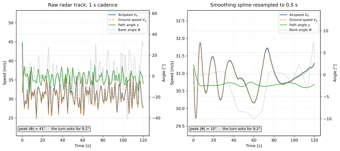

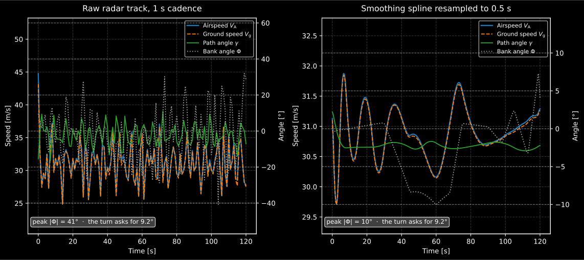
The same track, differentiated twice. The bank angle is derived from the curvature, which is a second derivative of position, so a few metres of radar noise at a 1 s cadence turn a 9.2° turn into 41° of nonsense — and the emission frame is tilted by that angle, so the error goes straight into the source level. After spline resampling to 0.5 s the trace shows one clean trough through the turn, peaking at 10° against the 9.2° the geometry asks for. Smooth before you differentiate.

Show the code for this figure

import matplotlib.pyplot as plt
import numpy as np
from scipy.interpolate import UnivariateSpline
from phonometry import aircraft

rng = np.random.default_rng(20260808)
t_true = np.arange(0.0, 120.001, 0.1)
speed, radius, sigma = 30.87, 600.0, 4.0          # 60 kt, a 600 m turn, 4 m noise
turn = np.clip((t_true - 40.0) / (radius / speed), 0.0, np.pi / 2)
xy = np.column_stack([np.cumsum(np.cos(turn)), np.cumsum(np.sin(turn))]) * speed * 0.1
t_radar = np.arange(0.0, 120.001, 1.0)
raw = np.column_stack([np.interp(t_radar, t_true, xy[:, 0]),
                       np.interp(t_radar, t_true, xy[:, 1]),
                       300.0 - 1.2 * t_radar]) + rng.normal(0.0, sigma, (121, 3))
t_fine = np.arange(0.0, 120.001, 0.5)
smooth = np.column_stack([
    UnivariateSpline(t_radar, raw[:, k], s=t_radar.size * sigma ** 2)(t_fine)
    for k in range(3)])

fig, axes = plt.subplots(1, 2, figsize=(12, 5.4))
for ax, times, pos in ((axes[0], t_radar, raw), (axes[1], t_fine, smooth)):
    aircraft.flight_path_kinematics(times, pos).plot(ax=ax)
plt.show()

The single event: SEL, LASmax and EPNL

rotorcraft_event_level runs the whole chain for one flyover at one receiver: per track point the flight condition selects (or blends) the hemispheres, the emission angles address the source level (the frame is oriented by the heading and tilted by the bank angle in turns; pitch attitude is implicit in the hemispheres), and the received one-third-octave history is expressed at recorded time $t_r=t_e+r/c$ (Eq. 22, $c=346.1\text{m/s}$) and integrated: LASmax, SEL over the full history and over the certification 10 dB-down window (Doc 32 Eq. 27), and EPNL per ICAO Annex 16 (Doc 32 Eq. 28).

res = aircraft.rotorcraft_event_level(
    hemispheres, speeds, angles,      # the database
    times, positions,                 # the track (m, z up)
    receiver=(120.0, 0.0),            # ground position of the microphone
    ground=aircraft.RotorcraftGround(flow_resistivity="D"))   # grass site
res.la_max, res.sel, res.epnl         # LASmax, SEL, EPNL
res.plot()                            # the LA(t) time history

Three numbers of the same event, and they are not interchangeable. LASmax is one instant: the largest A-weighted level of the history, and nothing about how long the event lasted. SEL integrates the whole history and normalises it to one second, so it exceeds LASmax by an amount that grows with slant distance and falls with speed — for the level flyover below, 60 kt at 150 m over a 120 m sideline, the gap is 10.3 dB; halve the speed and it grows to 12.2 dB, double the height and it grows to 12.5 dB. EPNL is a different animal: it is built from noy-weighted spectra with a tone correction over the 10 dB-down window (Doc 32 Eq. 28, running the Annex 16 Appendix 2 chain), so it is not comparable with either — for the same event it reads 91.2 EPNdB against a SEL of 88.8 dB(A). Use LASmax and SEL for contour and annoyance work, and EPNL only against certification levels.

The shape of the history is worth reading too. Each emission is stamped at recorded time $t_r=t_e+r/c$, and $r$ is largest far from the closest point of approach and smallest at it, so the received history is compressed on the way in and stretched on the way out — the curve is asymmetric before any directivity is involved. Where LASmax actually falls then depends on the hemisphere: with the mildly forward-lobed one below it arrives about a second before the sound emitted at the closest point of approach, because the loudest emission direction is reached slightly before abeam. That is the reason the method carries a hemisphere rather than a source level.

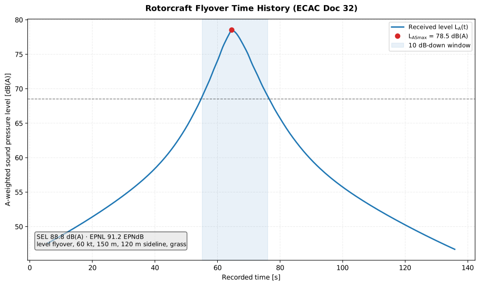
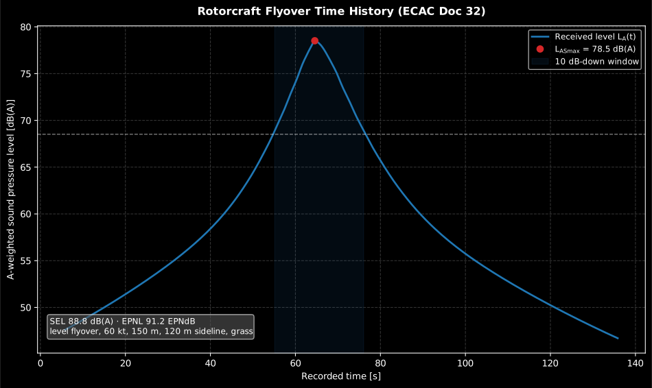
Two asymmetries in one curve, and neither is a modelling artefact. $L_{AS,max}$ = 78.5 dB(A) arrives at 64.56 s, a full second before the sound emitted at the closest point of approach (65.56 s), because the hemisphere’s loudest direction is reached slightly before abeam. And the 10 dB-down window runs 9.4 s up and 11.5 s down about the peak — the retarded time compresses the approach and stretches the departure. Integrating all 20.9 s of it and normalising to one second gives SEL = 88.8 dB(A), 10.3 dB above the peak the meter would show.

Show the code for this figure

import matplotlib.pyplot as plt
import numpy as np
from phonometry import aircraft

# A synthetic helicopter-like hemisphere on the standard 31-band, 10° grid.
freqs = 1000.0 * 10.0 ** (np.arange(-20, 11) / 10.0)   # 10 Hz-10 kHz thirds
az = np.arange(-90.0, 91.0, 10.0)
po = np.arange(0.0, 181.0, 10.0)
spectrum = 88.0 - 12.0 * np.log10(freqs / 100.0) ** 2   # broad low-mid hump
levels = (spectrum[None, None, :] - 0.045 * np.abs(po - 80.0)[None, :, None]
          - 0.02 * np.abs(az)[:, None, None])
h = aircraft.RotorcraftHemisphere(freqs, az, po, levels)

speed = 30.87                                           # 60 kt, in m/s
t = np.arange(0.0, 130.01, 0.5)
track = np.column_stack([np.zeros_like(t), speed * (t - 65.0),
                         np.full_like(t, 150.0)])
event = aircraft.rotorcraft_event_level(
    [h], [speed], [0.0], t, track, (120.0, 0.0),
    ground=aircraft.RotorcraftGround(flow_resistivity="D"))
event.plot()
plt.show()

Radar-track workflows can hand the smoothed per-point airspeed, path_angle, heading and bank_angle of a RotorcraftTrackState directly instead of deriving them from the positions; when they are derived, the track is in metres and seconds, so the database airspeeds must then be in m/s.

Ground-grid contours

rotorcraft_noise_contour evaluates the same event over a whole grid in one vectorised pass per emission step and reduces each receiver’s history to the SEL (metric="exposure") or LASmax (metric="maximum") footprint:

import numpy as np
from phonometry import aircraft

res = aircraft.rotorcraft_noise_contour(
    hemispheres, speeds, angles, times, positions,
    x=np.linspace(-2000.0, 2000.0, 81),
    y=np.linspace(-3000.0, 3000.0, 121),
    metric="exposure",
    ground=aircraft.RotorcraftGround(flow_resistivity="D"))
res.plot()                            # filled SEL contours

The ground may vary across the receivers without a full elevation model: the flow_resistivity and ground_elevation of the RotorcraftGround accept one value per grid point (shape (len(y), len(x))), and each receiver’s two-ray model then uses its local values.

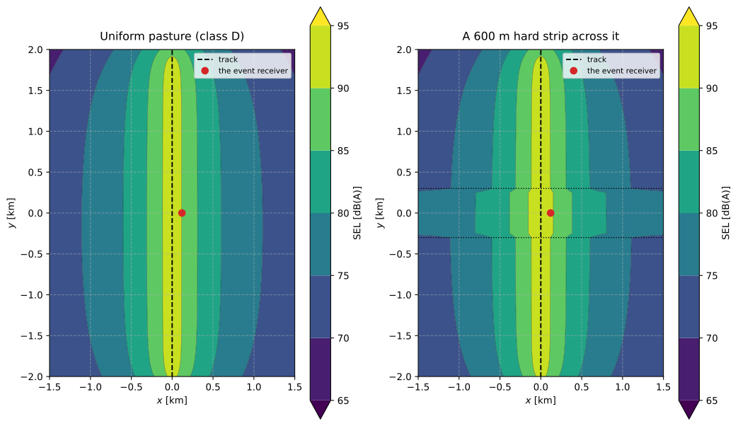
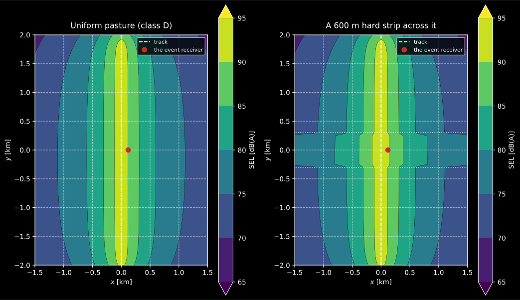
The deliverable of the whole method, and what the ground does to it. Over uniform pasture the footprint is a band along the track, its width set by the hemisphere and the slant distance. Give the same run a 600 m hard strip across the track — an apron, a runway, a lake — and every contour steps outward inside it, because the reflection stops being absorbed. That step is the per-receiver flow_resistivity map doing its work; a study that leaves the default "G" in place is drawing the right-hand picture everywhere.

Show the code for this figure

import matplotlib.pyplot as plt
import numpy as np
from phonometry import aircraft

x = np.linspace(-1500.0, 1500.0, 61)
y = np.linspace(-2000.0, 2000.0, 81)
sigma = np.where(np.abs(y)[:, None] < 300.0, 20.0e6,        # the hard strip
                 np.full((y.size, x.size), 200.0e3))        # pasture elsewhere

fig, axes = plt.subplots(1, 2, figsize=(11, 6.4))
for ax, ground in ((axes[0], aircraft.RotorcraftGround(flow_resistivity="D")),
                   (axes[1], aircraft.RotorcraftGround(flow_resistivity=sigma))):
    res = aircraft.rotorcraft_noise_contour(
        [h], [speed], [0.0], times, positions, x=x, y=y,
        metric="exposure", ground=ground)
    res.plot(ax=ax)                      # the plot works in kilometres
    ax.plot(positions[:, 0] / 1000.0, positions[:, 1] / 1000.0, "k--", lw=1.4)
plt.show()

Terrain: the mean ground plane and screening

Doc 32, 1st ed. assumes flat terrain. The EASA NORAH2 modelling guidance (Olsen et al. 2024), which the rest of this page follows at equation level, adds the machinery for real sites. A varying vertical section is represented by its mean ground plane (Eq. 36-40), the least-squares line through the terrain polyline computed in closed form; source and receiver enter the flat-ground equations with their equivalent heights, measured orthogonally to that plane and floored at 0.1 m. Ground that changes type along the path averages its flow resistivity by the logarithm, weighted by segment length (Eq. 41).

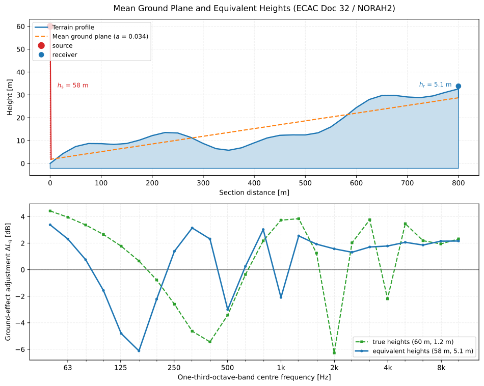
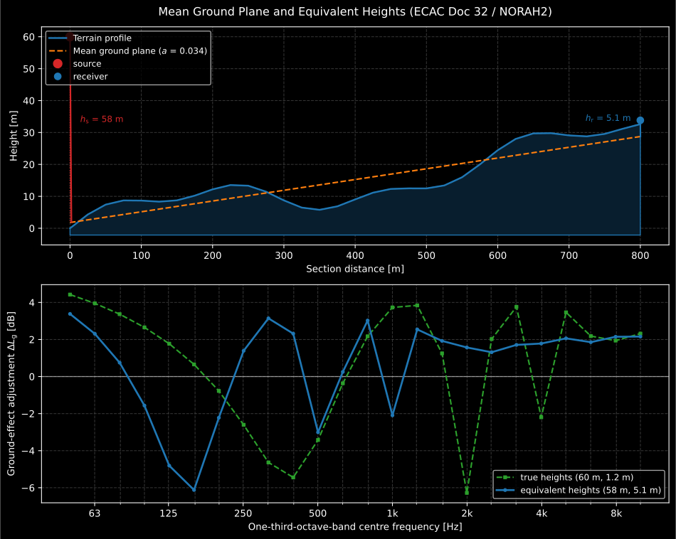
Why the construction exists. The receiver stands 1.2 m above the terrain, but the terrain under it is 4 m above the plane the section fits, so its equivalent height is 5.1 m — and the ground effect is a function of the equivalent heights, not the true ones. Four metres of local relief move the first interference minimum by an octave. The 0.1 m floor exists for the opposite case, a receiver in a hollow that the fitted plane passes above.

Show the code for this figure

import matplotlib.pyplot as plt
import numpy as np
from phonometry import aircraft

d = np.linspace(0.0, 800.0, 33)
z = 0.035 * d + 6.0 * np.sin(d / 90.0) + 2.5 * np.sin(d / 31.0)
plane = aircraft.mean_ground_plane(d, z)
m, c = float(plane.slope), float(plane.intercept)

def equivalent(point):
    """Height measured orthogonally to the fitted plane, floored at 0.1 m."""
    return max(abs(point[1] - m * point[0] - c) / np.hypot(1.0, m), 0.1)

src, rcv = (0.0, 60.0), (800.0, float(z[-1]) + 1.2)
freqs = 1000.0 * 10.0 ** (np.arange(-13, 11) / 10.0)
fig, (ax, ax2) = plt.subplots(2, 1, figsize=(10, 8))
plane.plot(ax=ax)
for heights, style in (((src[1] - z[0], 1.2), "--"),
                       ((equivalent(src), equivalent(rcv)), "-")):
    ax2.semilogx(freqs, aircraft.ground_effect_adjustment(
        freqs, heights[0], heights[1], rcv[0], flow_resistivity="D"), style)
plt.show()

When terrain blocks the line of sight, the sound follows the shortest convex path over it (the NORAH2 guidance calls it the rubber band) and every touched vertex is a diffraction edge. The attenuation combines the pure diffraction of the path difference $\delta$ (Eq. 42-44, $10C_h{\log }_{10}(3+(40/\lambda )C^{\prime \prime }\delta )$, capped at 25 dB) with the source-side and receiver-side ground effects, each over its own mean ground plane and weighted by its image-path diffraction (Eq. 45-47, the CNOSSOS-EU scheme the NORAH2 guidance adopts). The ground effect is not evaluated separately in that regime.

Whether any of that is worth paying for is a question about wavelengths. Screening is governed by the path difference over the obstacle measured in wavelengths — the attenuation grows with $\delta /\lambda$ and is capped at 25 dB — so a metre of path difference is worth little at 100 Hz and a great deal at 4 kHz. For a rotorcraft the geometry rarely arises at all: the source is normally hundreds of metres up, so the line of sight is broken only for receivers far to the side or behind ridges, which is precisely where the levels are already low. Near the track, terrain acts through the mean plane and the equivalent heights above, not by screening. The practical rule is to run one section with terrain_screening_adjustment at the worst-looking receiver first, and only pay for a full elevation model if that section turns out to be screened.

from phonometry import diffraction_attenuation

bands = [63.0, 250.0, 1000.0, 4000.0]
diffraction_attenuation(bands, 0.0, edge_height=2.5)   # grazing incidence
diffraction_attenuation(bands, 1.0, edge_height=2.5)   # 1 m into the shadow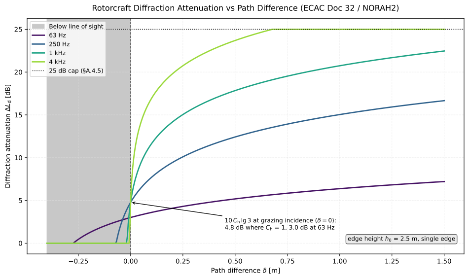

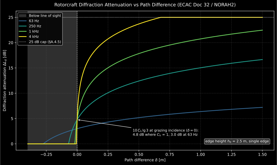
A single number tells the whole story only when both the wavelength and $C_h$ are fixed: the 4 kHz curve is already at the 25 dB cap by $\delta$ = 0.68 m, the 1 kHz curve is still climbing at $\delta$ = 1.5 m (22.5 dB, short of the cap), and the 63 Hz curve reaches only 7.2 dB there, held back by its own $C_h$ = 0.63 (Eq. 43, $h_0$ = 2.5 m) on top of the longer wavelength. At grazing incidence the three bands whose $C_h$ = 1 cross 4.8 dB, but 63 Hz crosses at 3.0 dB instead, because that value scales with $C_h$ too, not with wavelength alone.

Show the code for this figure

import matplotlib.pyplot as plt
import numpy as np
from phonometry import diffraction_attenuation

bands = np.array([63.0, 250.0, 1000.0, 4000.0])
delta = np.linspace(-0.4, 1.5, 441)
ld = np.array([diffraction_attenuation(bands, float(d), edge_height=2.5)
              for d in delta])

fig, ax = plt.subplots(figsize=(9, 6))
for i, label in enumerate(["63 Hz", "250 Hz", "1 kHz", "4 kHz"]):
    ax.plot(delta, ld[:, i], label=label)
ax.axvline(0.0, color="0.5", linestyle="--")
ax.axhline(25.0, color="0.5", linestyle=":", label="25 dB cap")
ax.set(xlabel="Path difference δ [m]",
       ylabel="Diffraction attenuation ΔLd [dB]")
ax.legend()
plt.show()

mean_ground_plane, mean_flow_resistivity and diffraction_attenuation expose the pieces; terrain_screening_adjustment runs the whole section:

import numpy as np
from phonometry import aircraft

d = [0.0, 150.0, 260.0, 300.0, 340.0, 420.0, 600.0]     # section distances
z = [0.0, 4.0, 48.0, 62.0, 40.0, 8.0, 2.0]              # terrain heights
freqs = 1000.0 * 10.0 ** (np.arange(-13, 11) / 10.0)
res = aircraft.terrain_screening_adjustment(
    freqs, source=(0.0, 90.0), receiver=(600.0, 3.2), distances=d, heights=z,
    flow_resistivity="D")
res.screened, res.path_difference      # True, the rubber-band delta
res.adjustment                         # per band, replaces the flat-ground ΔLg
res.plot()                             # the section geometry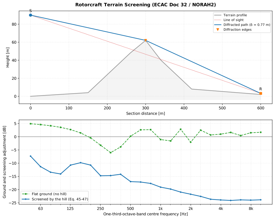

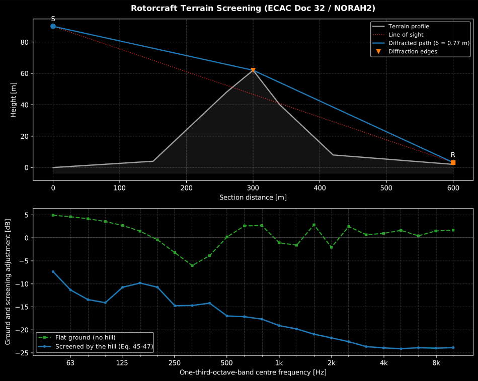
The hill is worth 0.766 m of path difference, and that single number is the whole spectrum. It is a ninth of a wavelength at 50 Hz and nearly nine wavelengths at 4 kHz, so the screened curve reads −7.3 dB in the lowest band and saturates near the 25 dB cap from about 2.5 kHz up — 23.9 dB at 4 kHz. Read against the flat-ground comb, the hill buys 12.3 dB at 50 Hz and about 25 dB across the top of the range. Terrain screening is a high-frequency instrument, and it does not fix a low-frequency complaint.

Show the code for this figure

import matplotlib.pyplot as plt
import numpy as np
from phonometry import aircraft

freqs = 1000.0 * 10.0 ** (np.arange(-13, 11) / 10.0)   # 50 Hz-10 kHz thirds
d = np.array([0.0, 150.0, 260.0, 300.0, 340.0, 420.0, 600.0])
z = np.array([0.0, 4.0, 48.0, 62.0, 40.0, 8.0, 2.0])
res = aircraft.terrain_screening_adjustment(
    freqs, (0.0, 90.0), (600.0, 3.2), d, z, flow_resistivity="D")
flat = aircraft.ground_effect_adjustment(freqs, 90.0, 1.2, 600.0,
                                         flow_resistivity="D")

fig, (ax, ax2) = plt.subplots(2, 1, figsize=(9, 7))
res.plot(ax=ax)
ax2.axhline(0.0, color="0.5", linewidth=1.0)
ax2.semilogx(freqs, flat, ls="--", marker="s", markersize=3,
             label="Flat ground (no hill)")
ax2.semilogx(freqs, res.adjustment, marker="o", markersize=3,
             label="Screened by the hill (Eq. 45-47)")
ax2.set(xlabel="One-third-octave-band centre frequency [Hz]",
        ylabel="Ground and screening adjustment [dB]")
ax2.grid(True, which="both", alpha=0.3)
ax2.legend()
plt.show()

The event and contour run over real sites by passing a digital elevation model in the RotorcraftGround: terrain=(x, y, z) on the track frame. Every emission-receiver pair then samples its own vertical section at terrain_resolution (default: the model’s cell size) and evaluates it with the machinery above; the receiver ground comes from the model. The cost grows with track points times grid points, so keep contour grids modest with terrain.

res = aircraft.rotorcraft_event_level(
    hemispheres, speeds, angles, times, positions, receiver=(1200.0, 300.0),
    ground=aircraft.RotorcraftGround(terrain=(tx, ty, tz),
                                     flow_resistivity="D"))

Validation

The implementation is anchored on the NORAH2 guidance Table 4 (all 31 bands), the closed-form inverse-square spreading, the analytic rigid-ground and grazing limits of the ground effect, off-node bilinear lookups on the reference hemispheres of all eleven rotorcraft types, hand-checked interpolation simplices, closed-form kinematics and the Lorentzian $\mathrm{SEL}-L_{ASmax}$ flyover integral. End to end it reproduces the NORAH2 prototype’s ARP verification cases:

Quantity	Oracle	Agreement
Band levels, 31 bands	NORAH2 guidance Table 4	exact
Emission angles	NORAH2 prototype, ARP cases	0.01°
Retarded time	same	0.02 s
Per-step level, hard ground, to 18 km	same	0.08 dB(A)
$L_{ASmax}$	same	0.03 dB
SEL	same	0.05 dB hard ground, 0.4 dB soft
Contour grid, 187 microphones	ARP Case 3	0.7 dB worst case
$\mathrm{PNLTM}$	same	0.1 dB
EPNL	same	≈ 1.3 dB (see below)
Hover LASmax/SEL, 8 microphones	ARP Case 4 (out-of-ground hover)	0.45 dB worst case

Two caveats, not rounding

The EPNL agreement is an order of magnitude looser than everything else because the prototype applies a sub-noy-floor perceived-noisiness policy that differs from the published Annex 16 law; the divergence is in the reference, not in the chain.

At far range over soft ground the prototype damps the coherent two-ray interference of guidance Eq. 30 towards the incoherent sum, which reaches 4.9 dB on individual low-level steps beyond 7 km. Neither Doc 32 nor the NORAH2 guidance contains such a term, so this implementation follows the published equations and does not reproduce it.

The Table 3 derivation is additionally anchored in closed form (the ring-to-rim identity, hand-computed constant-φ bins, the exact Approach 3 offsets), and the hover row of the table is the prototype’s out-of-ground hover case reproduced with the prototype’s own conventions passed explicitly: mapping="bearing" and its +8 dB database correction as offset_db. Its eight microphones span bearings, elevations, receiver heights from 0.01 m to 8.2 m and four flow resistivities; the residual peaks on the nadir microphones, where the prototype’s damped interference differs most from the published coherent Eq. 30.

The terrain machinery is anchored in closed form: the mean ground plane is exact on linear and symmetric profiles, a flat section reproduces the flat-ground model to machine precision and an inclined plane its analytic rotation, the log-mean resistivity recovers the geometric mean, the grazing diffraction gives the classical $10{\log }_{10}3$, and a hand-checked hill fixes the rubber-band path difference. Per-receiver ground handling validates end to end against the prototype’s ARP Case 3 (187 microphones, each on its own ground elevation: every step level to 0.08 dB(A), SEL/LASmax to 0.05 dB, the contour grid to 0.15 dB) and the mixed-ground Case 2 grid reproduces in a single per-receiver-resistivity call. The prototype’s public release does not include a reconstructible screening case (the frame of its terrain model could not be pinned to the published outputs), so the diffraction chain itself rests on the closed-form anchors and its CNOSSOS-EU lineage.

What this guide covers

• Covered

  The ECAC Doc 32 hemisphere method and the EASA NORAH2 equation- level guidance (§A.3-A.5): the noise hemisphere and its bilinear lookup (RotorcraftHemisphere, hemisphere_source_level), the three propagation adjustments (spherical_spreading_adjustment, atmospheric_adjustment, ground_effect_adjustment, the Chien-Soroka model with Delany-Bazley impedance and the CNOSSOS flow-resistivity classes), the flight-condition interpolation (flight_condition_weights, interpolated_source_level), the hover, idle and taxi source derivation of Table 3 (hover_ring_hemisphere, hover_derived_hemisphere), the flight-path kinematics (flight_path_kinematics), the single-event SEL, LASmax and EPNL (rotorcraft_event_level), ground-grid contours (rotorcraft_noise_contour) and the terrain mean-ground-plane and diffraction-screening chain (mean_ground_plane, mean_flow_resistivity, diffraction_attenuation, terrain_screening_adjustment). Validated against the NORAH2 guidance Table 4, closed-form geometric and grazing limits, and end to end against the NORAH2 prototype’s ARP verification cases, including its out-of-ground-hover operation.

• Not covered

  The §A.3.5 fallback for a type with no hover data at all — two side-line level-flight microphones corrected to the 150 m hover circle by the ICAO Annex 16 integrated method — is a measurement-correction chain this module, which consumes already-reduced hemispheres, does not model. No hemisphere database ships with phonometry, and there is no NORAH file reader: the method is implemented, the data is not, so the arrays come from a measurement campaign or from the NORAH2 reference database and are assembled by the reader. Refraction by atmospheric gradients is outside Doc 32 itself, as is the flight-condition interpolation, which follows the NORAH2 guidance instead.

See also

• Aircraft noise: Effective Perceived Noise Level: the ICAO Annex 16 Appendix 2 chain this page’s Doc 32 Eq. 28 term calls, and the measurement practice a hemisphere campaign follows.
• Airport Noise (ECAC Doc 29): the fixed-wing contour method, where a noise-power-distance table plays the role the noise hemisphere plays here.
• Outdoor sound propagation: the ISO 9613-2 ground effect and the CNOSSOS ground classes this two-ray adjustment shares.
• API reference: aircraft.rotorcraft_noise.

References

• Chien, C. F., & Soroka, W. W. (1975). Sound propagation along an impedance plane. Journal of Sound and Vibration, 43(1), 9-20. https://doi.org/10.1016/0022-460X(75)90200-XThe two-ray interference solution over an impedance plane behind the ground-effect adjustment.
• Delany, M. E., & Bazley, E. N. (1970). Acoustical properties of fibrous absorbent materials. Applied Acoustics, 3(2), 105-116. https://doi.org/10.1016/0003-682X(70)90031-9The one-parameter flow-resistivity impedance model the ground effect evaluates.
• European Civil Aviation Conference. (2026). Report on standard method of computing rotorcraft noise contours (ECAC.CEAC Doc 32, 1st ed.). The standard rotorcraft contour method whose hemisphere source model and propagation adjustments this page implements. The linked PDF is the free download; the document is catalogued on the ECAC documents page (https://www.ecac-ceac.org/documents/ecac-documents-and-international-agreements).
• Kephalopoulos, S., Paviotti, M., & Anfosso-Lédée, F. (2012). Common noise assessment methods in Europe (CNOSSOS-EU) (EUR 25379 EN). Publications Office of the European Union. https://doi.org/10.2788/31776The flow-resistivity ground classes 'A'-'H' accepted by ground_effect_adjustment.
• Olsen, H., Tuinstra, M., & van Oosten, N. (2024). Rotorcraft noise modelling guidance (Research Project NOISE SC01, deliverable D1.5d, contract EASA.2020.FC.06). European Union Aviation Safety Agency. The equation-level guidance (Eq. 13-35) behind the implementation, with the Table 4 attenuation values and the reference hemispheres used as oracles. Implemented scope (§A.3-A.5): the noise hemisphere, spherical spreading, atmospheric attenuation (ISO 9613-1, Table 4), the Chien-Soroka ground effect (Delany-Bazley impedance, CNOSSOS flow resistivity), the flight-condition interpolation (Eq. 3-10), the flight-path kinematics (Eq. 16-21 / Doc 32 Eq. 8-10), recorded time (Eq. 22), the single-event metrics SEL/LASmax and EPNL (Doc 32 Eq. 27/28, ICAO Annex 16 App. 2), the mean ground plane and equivalent heights (Eq. 36-40), the log-mean flow resistivity (Eq. 41), the terrain screening chain (Eq. 42-47 with the guidance's noise-path appendices; CNOSSOS-EU lineage) and the hover/idle source derivation of §A.3.5 Table 3 (ring-to-hemisphere constant-φ extension, Approach 2/3 offsets, taxi selection). Only §A.3.5's no-hover-data fallback (two side-line microphones corrected to the 150 m hover circle by the ICAO Annex 16 integrated method) remains outside the implementation. The linked PDF is the free download; the project is catalogued on the EASA project page (https://www.easa.europa.eu/en/research-projects/environmental-research-rotorcraft-noise).