The ANP fleet database
Standards: ECAC.CEAC Doc 29
Airport Noise (ECAC Doc 29) computes an event level from a noise-power-distance table and a flight path. That guide supplies both by hand, which is what you want while learning the method and what you never want afterwards: for a real study the numbers come from the Aircraft Noise and Performance (ANP) database that EASA and EUROCONTROL publish for the aircraft types actually flying.
That database ships with phonometry. This guide is the bridge between it and the Doc 29 functions: how to open it, what one aircraft record holds, and how to go from an aircraft identifier to an event level or a contour without writing a table yourself.
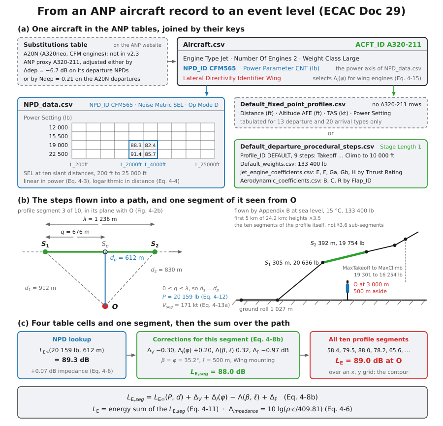
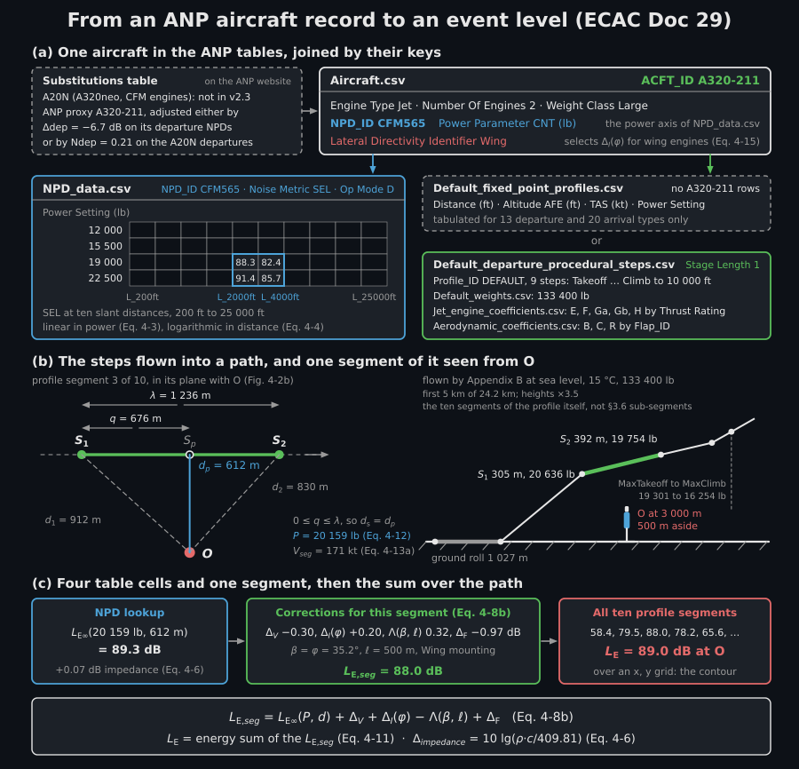
One aircraft, from its record to one number. A type the database lacks enters at the top, through a proxy the ANP website recommends and an adjustment you apply yourself. The A320-211 ships no fixed-point departure, so its published steps are flown at a sea-level aerodrome; the third of the ten profile segments that result passes 612 m from a receiver 3 km down the track and 500 m to the side, reads the four cells of the NPD table that surround 20 159 lb and 612 m, and at 88.0 dB carries about four fifths of the sound energy of the 89.0 dB event.
1. Opening the database
Section titled “1. Opening the database”load_anp_database() with no argument reads the copy shipped with the package.
Point it at a directory to read any other ANP CSV export instead.
from phonometry import aircraft
db = aircraft.load_anp_database()print(len(db.aircraft_ids))          # 155 aircraft typesac = db.aircraft("747100")print(ac.description)                # Boeing 747-100 / JT9DBDprint(ac.engine_type, ac.num_engines, ac.weight_class)print(ac.power_parameter, ac.mounting)
The sibling guides import the module as aircraft and call
aircraft.event_level(...) on it; here ac is one record out of the
database, and its event_level and noise_contour are those same functions
with the NPD tables and the default profile already filled in. Keeping the two
apart matters if you concatenate snippets from both pages.
An AnpAircraft describes itself with the engine type and count and the ICAO
wake weight class, and carries two fields you will use directly.
The power parameter names the quantity the NPD table is indexed by. It
matters because it is not a force in newtons but whatever the manufacturer
tabulated against, corrected net thrust in pounds for most jets, so a power you
pass to level has to be in those units.
The engine mounting is the one field of the record that the Doc 29 chain
itself reads. It is derived from the ANP lateral directivity identifier and is
one of "wing", "fuselage" or "propeller", which selects the
engine-installation correction that the
airport-noise guide applies by hand.
The choice is not cosmetic: at small depression angles wing and fuselage
mountings differ by more than a decibel, propellers take none of that
correction, and the shipped fleet splits 70 / 55 / 30 across the three. An
identifier the database does not recognise falls back to "wing".
Finding your aircraft
Section titled “Finding your aircraft”The identifiers are the ANP database’s own. They are close to an ICAO type
designator but not the same thing, because a type appears once per engine
variant: A320-232 is the IAE-engined A320 and 747100 the JT9D-engined
747-100. Search the descriptions to find yours rather than guessing the string:
from phonometry import aircraft
db = aircraft.load_anp_database()for aid in db.aircraft_ids:    rec = db.aircraft(aid)    if "A320" in rec.description:        print(aid, "|", rec.description, "|", rec.engine_type, "|", rec.mounting)# A320-211 | Airbus A320-211 / CFM56-5A1 | Jet | wing# A320-232 | Airbus A320-232 / V2527-A5 | Jet | wing
Match the engine variant before anything else: it changes the NPD levels by more than any of the per-segment corrections.
When your aircraft is not in the database
Section titled “When your aircraft is not in the database”Every real movement list contains types the database does not hold, and the
accepted remedy is substitution by an acoustically and operationally similar
type, not invention. Match on engine type and count first, then on weight class
and engine mounting, because those change the shape of the answer rather than
shifting it; check that the substitute’s power_parameter is the same quantity
as the original’s, since a table indexed by corrected net thrust in pounds
cannot take power settings computed for one indexed by anything else. Record the
substitution with the results (it is a modelling assumption, not a detail). The
same reasoning applies one level down: a type whose NPD curves are tabulated but
whose trajectory is not (see section 3) is usually better modelled with a
substitute trajectory and its own NPD table than by substituting the whole
aircraft.
2. The noise-power-distance curves
Section titled “2. The noise-power-distance curves”npd_curves returns the tabulated NPD surface for one operation ("D" for
departure, "A" for arrival) and one metric ("SEL" or "LAmax"): a level for
each combination of engine power setting and slant distance. Between the
tabulated nodes the Doc 29 interpolation is logarithmic in distance and linear
in power, which is what the curves below draw.
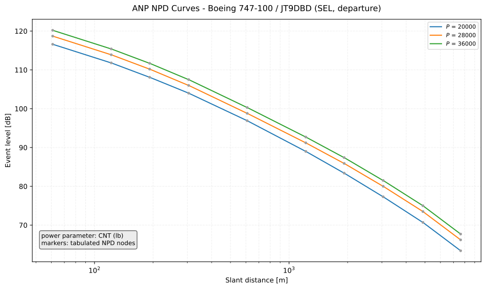
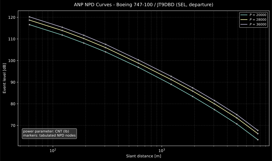
The three tabulated thrust settings are close to parallel: power mostly shifts the level, while distance sets the shape. The fall is close to the inverse-square rate at short range and steepens at long range as absorption accumulates, and the markers are the only distances at which the database asserts anything: everything between them is Doc 29 interpolation.
Show the code for this figure
import matplotlib.pyplot as pltfrom phonometry import aircraft
ac = aircraft.load_anp_database().aircraft("747100")curves = ac.npd_curves("D", "SEL")
fig, ax = plt.subplots(figsize=(10, 6))curves.plot(ax=ax)ax.set_title(f"ANP NPD Curves - {ac.description} (SEL, departure)")ax.text(0.02, 0.06,        f"power parameter: {ac.power_parameter}\n"        "markers: tabulated NPD nodes",        transform=ax.transAxes, va="bottom", fontsize=9)plt.show()
from phonometry import aircraft
aircraft.load_anp_database().aircraft("747100").npd_curves("D", "SEL").plot()To read a single value rather than draw the family, level interpolates at any
power and distance:
from phonometry import aircraft
curves = aircraft.load_anp_database().aircraft("A320-232").npd_curves("D", "SEL")print(curves.powers)                       # [10000. 14000. 19000. 23000.] lbprint(curves.level(19000.0, [304.8, 1000.0, 3000.0]))
The record’s power_parameter names those units: never assume newtons.
The distances are metres. The database tabulates them in feet, at the ten Doc 29 nodes from 200 ft to 25000 ft, and this bridge converts on read so everything downstream stays in SI.
3. The default trajectory
Section titled “3. The default trajectory”An aircraft record also carries default trajectories. profile returns one as a
Doc 29 flight path: an (N, 5) array of along-track, lateral and vertical
position plus the power setting and true airspeed, with boolean masks marking
which segments are the takeoff ground roll or the landing rollout.
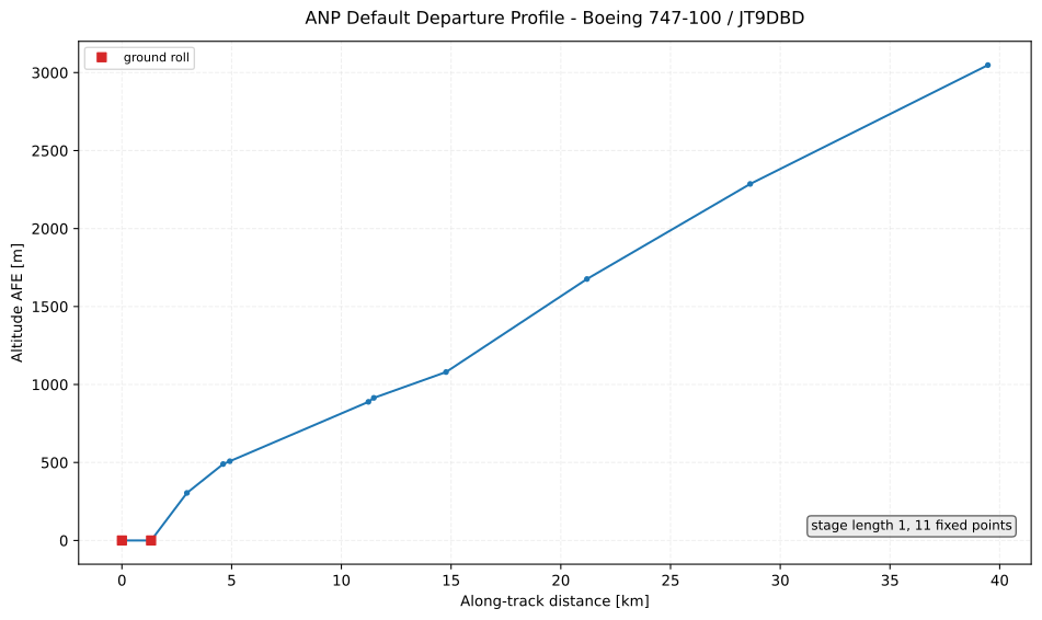
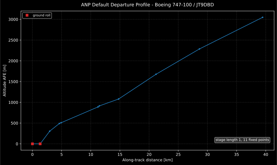
The first points sit at zero altitude and are the ground roll. What follows is the climb gradient, and it is the gradient rather than the level that decides the contour, because it fixes the slant distance at every receiver; the same aircraft at a longer stage length is heavier and climbs more slowly, so its footprint is longer and wider.
Show the code for this figure
import matplotlib.pyplot as pltfrom phonometry import aircraft
ac = aircraft.load_anp_database().aircraft("747100")profile = ac.profile("D", stage_length=1)
fig, ax = plt.subplots(figsize=(10, 6))profile.plot(ax=ax)ax.set_title(f"ANP Default Departure Profile - {ac.description}")ax.text(0.98, 0.06,        f"stage length {profile.stage_length}, "        f"{profile.path.shape[0]} fixed points",        transform=ax.transAxes, va="bottom", ha="right", fontsize=9)plt.show()
from phonometry import aircraft
aircraft.load_anp_database().aircraft("747100").profile("D", stage_length=1).plot()The stage length selects the trip-distance bin: a longer stage means more fuel, more weight and a shallower climb, so the same aircraft has one profile per bin. Doc 29 Vol. 2 Appendix G3.5 defines the bins by trip length in nautical miles: 1 is 0-500, 2 is 500-1 000, 3 is 1 000-1 500, 4 is 1 500-2 500, 5 is 2 500-3 500, 6 is 3 500-4 500, 7 is 4 500-5 500, and so on in 1 000 nmi steps to 10 (7 500-8 500), with 11 for anything longer and “M” for maximum range at maximum take-off mass. The take-off weight of each profile is computed at the bin’s representative range, defined as the minimum plus 70 % of the span, so bin 1 is weighed at 350 nmi and bin 4 at 2 200 nmi. Not every aircraft flies every bin, and the shipped fixed-point profiles cover stage lengths 1 to 7 for departures and 1 only for arrivals.
A fixed-point profile is a trajectory ready to fly, and most ANP entries do
not carry one: they describe their departures as procedural steps instead (climb
at this rate to that altitude, accelerate, retract flaps), which have to be flown
through a flight-mechanics performance model before they become a path. Of the
155 aircraft in the shipped database only 13 have a fixed-point departure
profile and 20 a fixed-point arrival profile; section 4 flies the rest. Asking
for a fixed-point profile that does not exist raises a KeyError naming the
stage lengths that do, which is also how to discover the bins an aircraft
actually ships:
from phonometry import aircraft
db = aircraft.load_anp_database()for identifier, operation, stage in (("A320-232", "D", 1), ("747100", "D", 9)):    try:        db.profile(identifier, operation, stage)    except KeyError as exc:        print(exc)# ... 'A320-232', operation 'D', stage length 1 (available stage lengths: [])# ... '747100', operation 'D', stage length 9 (available: [1, 2, 3, 4, 5, 6])
An empty list means the type has no fixed-point profile at all and needs a trajectory flown for it; a non-empty one means you asked for a bin this aircraft does not fly. NPD curves, on the other hand, are tabulated for every aircraft in the database.
4. Flying a published procedure
Section titled “4. Flying a published procedure”A procedure is not a trajectory, and that is the whole of the difficulty. Its steps say what the aeroplane does, not where it goes: climb at this rate to that altitude, accelerate to that speed, change to climb thrust. Where those instructions put it over the ground depends on the field, because the same steps flown from a hot runway high above sea level reach 10 000 ft much further out than from a cold one at the coast. There is nothing to tabulate, which is why the database ships the steps and not the points.
flight_profile flies them, through the ECAC Doc 29 Vol. 2 Appendix
B flight
performance model. It requires an aerodrome, because it computes the
trajectory and the trajectory depends on the field, where profile returns an
already tabulated fixed-point one and needs no such argument. It works in the
standard’s own units: feet, knots and pounds.
from phonometry import aircraft
sea_level = aircraft.Aerodrome(elevation_ft=0.0)flown = aircraft.load_anp_database().flight_profile(    "A320-211", "departure", aerodrome=sea_level, stage_length=1)print(len(flown.points), round(flown.distance_ft[-1]), flown.altitude_ft[-1])# 11 79423 10000.0flown.plot()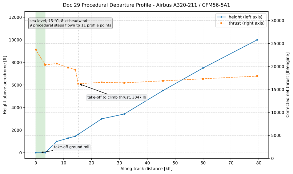
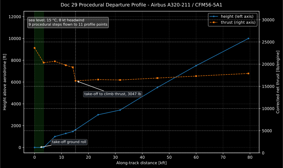
The A320-211 ships no fixed-point departure profile at all, so this is the only way to fly it. The shaded band is the take-off ground roll; the dotted line is where the procedure changes from take-off to climb thrust, a fall of 3 047 lb per engine that the height curve barely registers. That is what computing the thrust buys over reading a trajectory: nothing in the shape of the climb says the engines were throttled back, and the noise says it plainly.
Show the code for this figure
import matplotlib.pyplot as pltfrom phonometry import aircraft
db = aircraft.load_anp_database()airframe = db.aircraft("A320-211")profile = db.flight_profile(    "A320-211", "D", aerodrome=aircraft.Aerodrome(elevation_ft=0.0), stage_length=1)
fig, ax = plt.subplots(figsize=(10, 6))profile.plot(ax=ax)fig.axes[-1].set_ylim(0.0, 1.35 * float(profile.corrected_net_thrust_lb.max()))ax.set_title(f"Doc 29 Procedural Departure Profile - {airframe.description}", pad=12)plt.show()
procedural_profile crosses back into the units the noise chain speaks,
returning the same AnpProfile a fixed-point lookup does. event_level and
noise_contour take an aerodrome for the same reason, so an aircraft that
publishes only steps runs the whole Doc 29 chain from its identifier. That is
309 of the database’s 310 aircraft and operation pairs, against 33 with a
tabulated trajectory.
from phonometry import aircraft
hot_and_high = aircraft.Aerodrome(elevation_ft=5000.0, temperature_c=25.0)level = aircraft.load_anp_database().event_level(    "A320-211", [3000.0, 500.0, 0.0], "departure", aerodrome=hot_and_high)print(round(float(level.level), 1))    # 89.3 dB
One aerodrome, one atmosphere: the field’s temperature and pressure reach the
Doc 29 impedance adjustment as well as the performance model, so a profile flown
on a 35 °C day is not corrected for 15 °C by omission. temperature_c and
atmospheric_pressure_kpa still override it where the two genuinely differ.
5. Straight to an event level or a contour
Section titled “5. Straight to an event level or a contour”With both halves in the record, the aircraft can run the Doc 29 chain itself.
event_level places one flyover at a receiver, and noise_contour sweeps it
over a ground grid, each wiring the NPD curves and the default profile into the
functions the airport-noise guide builds by hand.
The observer is (x, y, z) in metres in the runway frame, and the origin
of that frame is not the airport boundary: runs along the runway centre
line with at start of roll for a departure and at the landing threshold
for an arrival, so arrival profiles carry negative on final approach. The
shipped data says it plainly: db.profile("747100", "D", 1).path[0] starts at
(brake release) and ends 39.5 km downrange, while
db.profile("707", "A", 1).path[0] starts at km and ends 1.5 km
past the threshold, so the two frames are nearly 35 km apart. is the lateral
offset from the extended centre line, positive to starboard of the direction of
travel; its sign is what selects the depression-angle branch of the
banked-segment rule. is the receiver height above local ground, left at 0 in
these examples where Doc 29 measures at 1.2 m, normally a difference under a
decibel.
Three arguments decide the rest, and two of them are silent. The metric
defaults to the sound exposure level, with "LAmax" available on request; the
stage length defaults to 1, the shortest trip-distance bin and therefore the
steepest climb and the smallest footprint; and the optional temperature_c and
atmospheric_pressure_kpa re-reference the tabulated levels from the reference
specific acoustic impedance to the air at the aerodrome, defaulting to the 15
°C and 101.325 kPa of the standard atmosphere. That last pair is a bookkeeping
term and not a weather correction: at the standard atmosphere it is worth +0.07
dB, and it rarely exceeds a few tenths. The NPD levels still carry the
absorption of the atmosphere they were reduced to, and the chain offers no
humidity-dependent band correction, so a hot dry aerodrome is not modelled by
passing its temperature.
from phonometry import aircraft
ac = aircraft.load_anp_database().aircraft("747100")flyover = ac.event_level([3000.0, 500.0, 0.0], "D")print(round(float(flyover.level), 1))     # 100.4 dB
That is the single-event sound exposure level of one 747-100 departure at a receiver 3 km down the track and 500 m to the side of it. Move the receiver out to 1 500 m lateral and it costs more than the extra distance alone, because the lateral attenuation switches on as the elevation angle falls below 50°.
import numpy as npfrom phonometry import aircraft
ac = aircraft.load_anp_database().aircraft("747100")contour = ac.noise_contour(    "D",    x=np.linspace(-2000.0, 12000.0, 40),    y=np.linspace(-3000.0, 3000.0, 30),)print(contour.levels.shape)      # (30, 40): one SEL per grid pointcontour.plot()
The grid is indexed (y, x), which is why the shape is (30, 40) and not the
other way round. The cheapest check that the grid and the path are in the same
frame is that the maximum of the array agrees with an event_level call at the
grid point where it occurs.
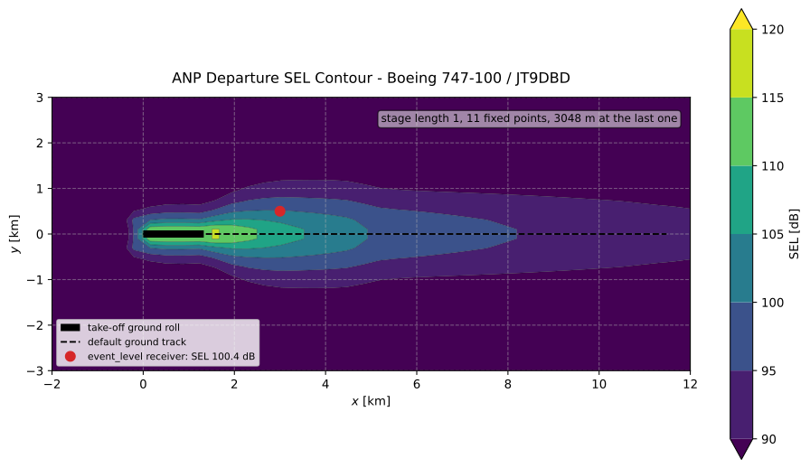
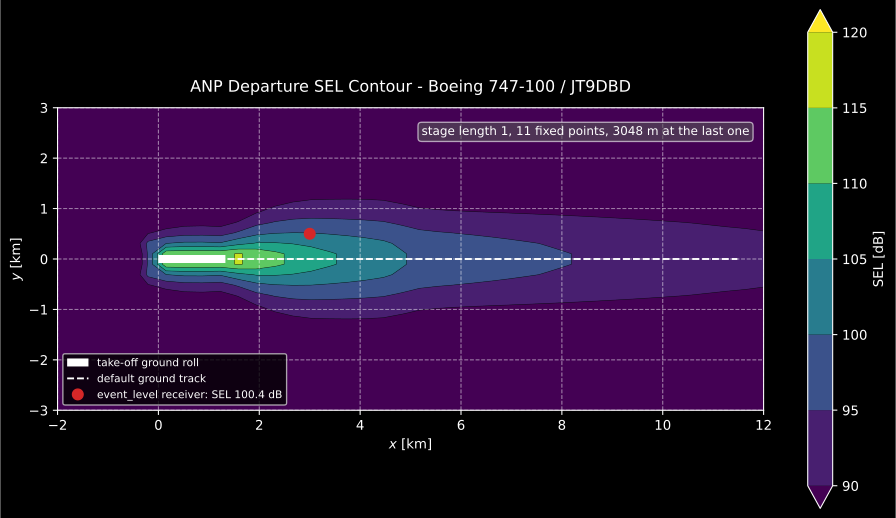
The real 747-100 footprint, from the database’s own NPD tables and default
departure profile: four lines of code, and nothing hand-written. It is narrower
and far more elongated than the teaching contour of the airport-noise guide,
because a real climb profile puts the aeroplane high quickly and the loud part
of the event stays close to the runway. The marked receiver is the
event_level call above, so the two halves of this section are the same
calculation at one point and at 1 200 of them.
Show the code for this figure
import matplotlib.pyplot as pltimport numpy as npfrom phonometry import aircraft
ac = aircraft.load_anp_database().aircraft("747100")profile = ac.profile("D", stage_length=1)x = np.linspace(-2000.0, 12000.0, 40)y = np.linspace(-3000.0, 3000.0, 30)
fig, ax = plt.subplots(figsize=(10, 5.5))ac.noise_contour("D", x=x, y=y).plot(ax=ax)      # the plot works in kilometresinside = profile.path[:, 0] <= x.max()ax.plot(profile.path[inside, 0] / 1000.0, profile.path[inside, 1] / 1000.0,        "k--", lw=1.4, label="default ground track")ax.plot([3.0], [0.5], "o", ms=8,        label=f"event_level receiver: SEL {float(flyover.level):.1f} dB")ax.set_xlim(x.min() / 1000.0, x.max() / 1000.0)ax.set_ylim(y.min() / 1000.0, y.max() / 1000.0)ax.legend(loc="lower left", fontsize=8)plt.show()
Everything these two return is the same result type the airport-noise guide uses, so the plotting, the contour extraction and the per-segment breakdown all work unchanged.
What this guide covers
Section titled “What this guide covers”Covered
Opening the shipped EASA ANP database (or another ANP CSV export) with
load_anp_database; what one aircraft record holds, including the power parameter its NPD table is indexed by and the engine mounting the Doc 29 chain reads; reading and interpolating the NPD surface withnpd_curvesandlevel; the default fixed-point trajectories and their stage-length bins; and running the Doc 29 single-event level and ground-grid contour from an aircraft identifier throughevent_levelandnoise_contour.Covered
The procedural-step profiles, which are how most ANP entries describe a departure, through the ECAC Doc 29 Vol. 2 Appendix B flight performance model:
flight_profileflies a published procedure for an aerodrome and its weather, andprocedural_profilehands the result to the Doc 29 chain as the same flight path a fixed-point profile produces.Not covered
Nothing of the database’s own content: it is read, never written, and phonometry ships version 2.3 and does not update it.
References
Section titled “References”- European Civil Aviation Conference. (2016). Report on standard method of computing noise contours around civil airports, Volume 2: Technical guide (ECAC.CEAC Doc 29, 4th ed.). The NPD and profile conventions the database follows, and the single-event chain the aircraft records feed. The linked PDF is the free download; the volumes are catalogued on the ECAC documents page (https://www.ecac-ceac.org/documents/ecac-documents-and-international-agreements).
- European Union Aviation Safety Agency. (2020). Aircraft Noise and Performance (ANP) database, version 2.3. EASA / EUROCONTROL. The NPD tables, aircraft metadata and default fixed-point profiles this guide reads. The database is published by EASA and EUROCONTROL and shipped with phonometry; its provenance is recorded in aircraft/data/anp/PROVENANCE.md.