Aircraft noise: Effective Perceived Noise Level
Standards: ICAO Annex 16Doc 9501IEC 61265SAE ARP 5534SAE ARP 866B
The Effective Perceived Noise Level (EPNL) is the noise-certification metric for transport-category aircraft. It condenses a half-second one-third-octave spectral time history of a flyover into a single number, in EPNdB, through five steps of ICAO Annex 16, Vol. I, Appendix 2. This page covers the four primitives that build the metric and the IEC 61265 measurement-system verifier. Each quantity is validated against the worked examples of the ICAO Doc 9501 Environmental Technical Manual (ETM) Vol. I.
Every certification level on this page is asked for at one of the three reference points Annex 16 fixes around the runway, so it helps to see them before the mathematics.
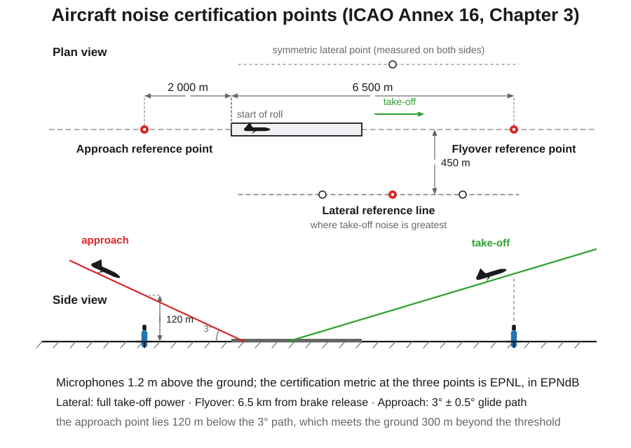
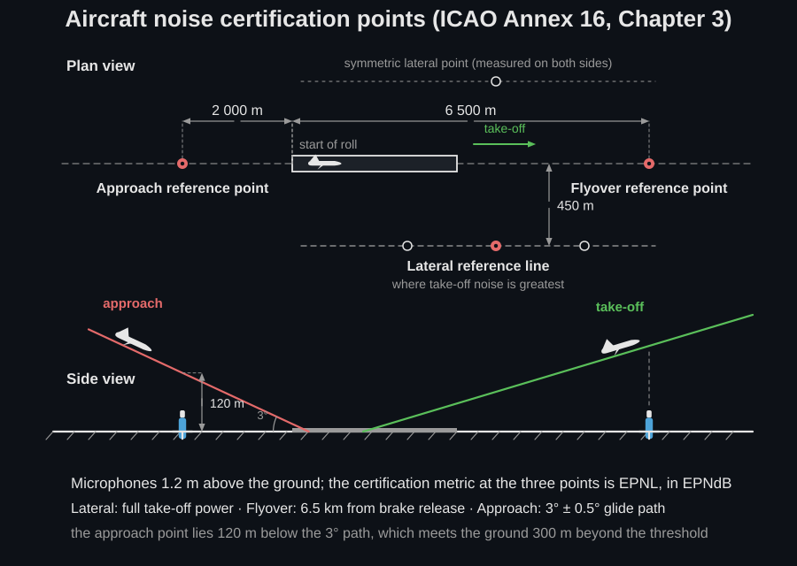
Three points, because a transport aeroplane is loud in three different ways. The lateral point, on a line 450 m to the side of the runway and placed where the take-off noise is greatest (§3.3.1 a), catches full take-off thrust at a shallow elevation angle, where ground effect and engine installation matter most. The flyover point, 6.5 km from the start of roll on the extended centre line, catches the aeroplane after thrust cutback, which is the community case. The approach point, 2 000 m before the threshold and 120 m below the 3° path, catches an airframe- and fan-dominated condition at low power. All three are scored with the EPNL of this page, but the limits differ and are not single numbers: Chapter 3 §3.4 sets them as lines rising with maximum certificated take-off mass: 101 EPNdB at flyover for a twin at 385 000 kg and above, 104 for a trijet and 106 for four engines or more, against 103 lateral and 105 on approach at the top of their own mass ranges. The same EPNL can pass at one point and fail at another. The microphone is 1.2 m above the ground at every point, which is why the measurement section below cares so much about grazing incidence.
Perceived noisiness and PNL
Section titled “Perceived noisiness and PNL”Each of the 24 one-third-octave-band levels (50 Hz–10 kHz) is converted to a perceived noisiness in noys by the analytic piecewise law of Table A2-3, then combined into the total noisiness and the perceived noise level .
A noy is a linear scale of perceived noisiness: two noys are meant to be twice as noisy as one, which is what lets the bands be combined arithmetically instead of energetically. The per-band conversion is piecewise-linear in level with slopes that differ from band to band, so the same 70 dB is worth far more noys at 3 kHz than at 63 Hz. The law carries the ear’s sensitivity in the same way an equal-loudness contour does, but calibrated on judgements of noisiness rather than loudness. The combination rule is a masking statement, not an energy sum: the loudest band alone accounts for 85 % of the total, and everything else together is credited with 15 %, which is why a single fan tone can dominate a spectrum that is broadband on paper. The logarithm then buys a level-like quantity: with , one noy is 40 PNdB and every doubling of total noisiness adds exactly 10 PNdB. Two limits come with it. The law is tabulated only for the 24 bands from 50 Hz to 10 kHz, so energy outside that range is invisible to EPNL by construction; and typical transport flyovers at the certification points land between about 90 and 110 PNdB, which is the scale a printed PNL should be read against.
from phonometry import aircraft
noys = aircraft.perceived_noisiness(spl)      # per-band noys (spl = 24 band levels, dB)pnl = aircraft.perceived_noise_level(spl)      # PNdB
Tone correction
Section titled “Tone correction”A pure tone is judged much noisier than the same energy spread across its one-third-octave band, so spectral irregularities (fan and turbine tones) are penalised by a tone correction . The slope (“encircling”) method reconstructs what the spectrum would look like without the tone by smoothing the band-to-band slopes into a background , so the excess is a tone-only quantity. Above 1.5 dB it is mapped to a correction factor by the rule of Table A2-2, and the maximum over bands is taken:
| Band | dB | dB | dB |
|---|---|---|---|
| 50 Hz-400 Hz and 6.3-10 kHz | dB | ||
| 500 Hz-5 kHz | dB |
The mid-band branch penalises a tone twice as hard, which is why a 2500 Hz fan tone dominates the correction of a turbofan spectrum. The implementation reproduces the ICAO Doc 9501 ETM Vol. I Table 3-7 turbofan example exactly ( at 2500 Hz).
Two traps come with the method. A rippled but tone-free spectrum can produce a correction, which the standard itself allows you to reject after a narrow-band re-analysis (§4.3.1 Step 10). And a tone falling between two bands splits its excess, so the raw correction comes out too small. The bandsharing adjustment , the shortfall of at the record against the mean of the records within one second of it, adds it back before the 10 dB-down window is located.
from phonometry import aircraft
c = aircraft.tone_correction(spl)              # dB; added to PNL to give PNLT# start_band=2 (80 Hz) is the aeroplane start of analysis; a helicopter# procedure starts at 50 Hz, which is what procedure="helicopter" selects in# effective_perceived_noise_level below.
Measuring the flyover
Section titled “Measuring the flyover”What goes into the chain is a time history of unweighted one-third-octave band sound pressure levels: 24 bands with nominal midband frequencies from 50 Hz to 10 kHz, one spectrum every 500 ms ± 5 ms (App. 2 §3.7.2). That cadence is prescribed, and the 10 s reference duration of the metric below is fixed independently of it, which is where the 13 dB constant of the uniform case comes from. A reader arriving with A-weighted data, or with a 1 s cadence, gets a plausible-looking number that is not an EPNL.
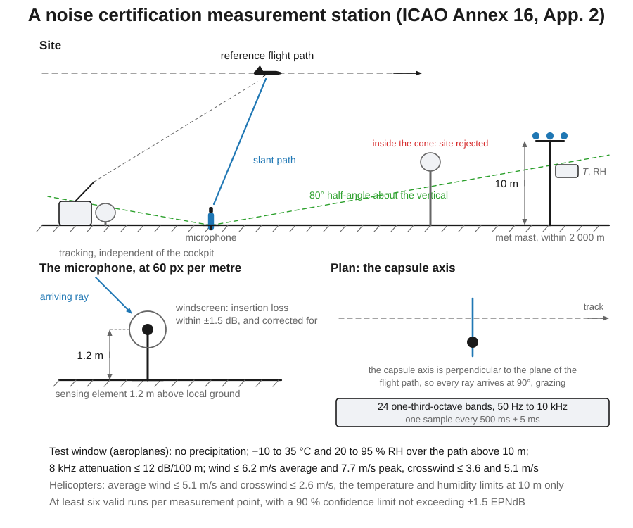
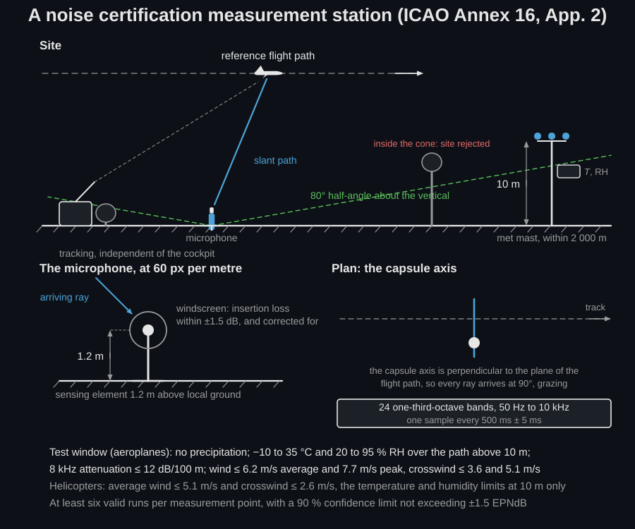
The station that produces those spectra is fixed clause by clause.
- The microphone. The sensing element sits 1.2 m above the local ground and is oriented for grazing incidence, with the element substantially in the plane defined by the predicted reference flight path and the station (§3.5.2). In practice the capsule axis points across the track, so sound arrives at 90° to it throughout the flyover. Its free-field sensitivity level must stay within ±1.0 dB of the calibration-check frequency from 50 Hz to 5 kHz and within ±2.0 dB at 6.3, 8 and 10 kHz (§3.5.3), and its directional response must meet Table A2-1 (§3.5.4). The windscreen’s insertion loss must stay inside ±1.5 dB over the same range at grazing incidence (§3.4) and is corrected for.
- The site. Relatively flat terrain with no excessive sound absorption (no thick, matted or tall grass, shrubs or wooded areas), and no obstruction that significantly influences the sound field inside a cone of 80° half-angle about the vertical through the microphone (§2.2.1). The people taking the measurement count as obstructions.
- The window. For aeroplanes: no precipitation; −10 °C to 35 °C and 20 % to 95 % relative humidity over the propagation path between 10 m and the aircraft; the 8 kHz attenuation coefficient no more than 12 dB/100 m over that path; average wind at 10 m no more than 6.2 m/s with a maximum of 7.7 m/s, and average crosswind no more than 3.6 m/s with a maximum of 5.1 m/s (§2.2.2.4.1). For helicopters the wind limits tighten to 5.1 m/s and 2.6 m/s and the temperature and humidity limits apply at 10 m only. Temperature, humidity, wind speed and direction are measured at 10 m above the ground within 2 000 m of the noise measurement point (§2.2.2.2).
- The tracking. Aircraft position is determined by a method independent of the cockpit flight instrumentation and time-synchronised with the acoustic record over at least the interval in which the noise is within 10 dB of (§2.3.1-2.3.2), the window the metric integrates over.
- The repetition. At least six valid runs per measurement point, and the sample must be large enough that the 90 % confidence limit on the average does not exceed ±1.5 EPNdB (§5.4.2).
Over the flyover, and its maximum is . The metric converts the tone-corrected level back to energy, sums it over the records between the two 10 dB-down points and divides by a fixed reference duration (App. 2 §4.6),
so EPNL is the level of a hypothetical 10 s exposure carrying the same noisiness-weighted energy as the real event. For the uniform half-second cadence this collapses to , the 13 dB being . The fixed reference duration is what makes a correction rather than an integral: a flyover that lingers near its peak for much longer than 10 s scores above , and one that sweeps past scores below it. In the ETM Vol. I Table 4-4 example the peak is PNdB, the 10 dB-down window runs from record 4 to record 28 of 31 and spans 10.2 s of increments, and the result is dB and EPNdB, just below because the window is barely longer than the reference duration.
That chain has an order to it, and the order is the part a finished time history cannot show. The tone correction is measured on each spectrum as it arrives, one record at a time, by fitting a background under the spectrum and reading the excess of the tone over it; the 10 dB-down window, by contrast, cannot be placed until the whole pass is over, because its two edges are defined relative to a peak that is not known until the last record has been taken. The clip runs a synthetic flyover in that order:
Forty-one one-third-octave spectra arrive at half-second intervals as an aircraft passes a microphone. On each spectrum a dashed background is fitted under the 2500 hertz fan tone and a double arrow measures the tone's excess over it, which at the peak reaches a correction of 3.97 decibels. Beside it two level histories are written point by point: the perceived noise level and, shaded above it, the tone-corrected level that exceeds it by that correction, rising to a peak of 120.57 PNdB as the aircraft reaches the microphone. Only once the pass has ended is the peak known; a dotted line then appears 10 decibels below it, the integration window fills between records 16 and 24, and the duration correction of -6.56 decibels and the final EPNL of 114.01 EPNdB appear last.
Forty-one one-third-octave spectra arrive at half-second intervals as an aircraft passes a microphone. On each spectrum a dashed background is fitted under the 2500 hertz fan tone and a double arrow measures the tone's excess over it, which at the peak reaches a correction of 3.97 decibels. Beside it two level histories are written point by point: the perceived noise level and, shaded above it, the tone-corrected level that exceeds it by that correction, rising to a peak of 120.57 PNdB as the aircraft reaches the microphone. Only once the pass has ended is the peak known; a dotted line then appears 10 decibels below it, the integration window fills between records 16 and 24, and the duration correction of -6.56 decibels and the final EPNL of 114.01 EPNdB appear last.
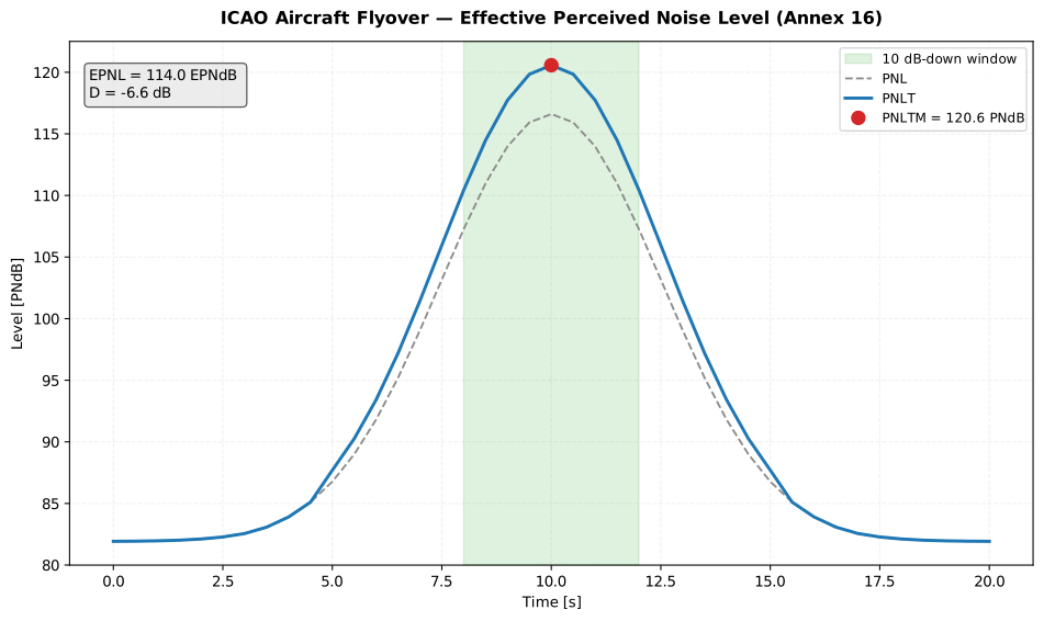
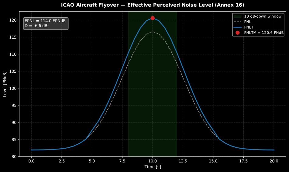
Two corrections, both visible. The gap between PNL and PNLT is the tone correction, worth 3.97 dB at the peak here because a 2500 Hz fan tone stands above its neighbours, which is why = 120.57 PNdB sits above the 116.61 PNdB the plain PNL reaches. The shaded 10 dB-down window spans records 16 to 24, about 4 s, well short of the fixed 10 s reference, so the duration correction is dB and = 114.01 EPNdB lands below the peak. A slower flyover over the same peak would score above it.
import numpy as npfrom phonometry import aircraft
# spectra: a (K, 24) array of one-third-octave band levels sampled every dt s,# here the synthetic flyover of the figure abovek, dt = 41, 0.5idx = np.arange(k)shape = 15.0 * np.exp(-((np.log10(aircraft.NOY_BANDS) - np.log10(400.0)) ** 2) / 0.5)gain = 30.0 * np.exp(-((idx - 20.0) ** 2) / (2 * 5.0**2)) - 5.0spectra = (55.0 + shape)[None, :] + gain[:, None]spectra[:, 17] += 12.0 * np.exp(-((idx - 20.0) ** 2) / (2 * 6.0**2))  # 2500 Hz fan tone
res = aircraft.effective_perceived_noise_level(spectra, dt=0.5)print(res.epnl, res.pnltm, res.duration_correction, res.band_limits)res.plot()   # PNL/PNLT time history (needs matplotlib)
effective_perceived_noise_level returns an EPNLResult bundling the per-record
pnl, tone_correction, pnlt, the peak pnltm, the bandsharing_adjustment,
the duration_correction, the epnl and the 10 dB-down band_limits. Its
procedure= argument starts the analysis at 80 Hz for an aeroplane (the
default) and at 50 Hz for a helicopter, and dt may be a per-record array
rather than a scalar, which is how the variable increments of the integrated
method enter. The reference-condition integrated-method example of ETM Vol. I
Table 4-4 (a different, real certification time history, with increments
between 0.395 s and 0.431 s) is reproduced as
.
Show the code for this figure
aircraft.effective_perceived_noise_level(spectra, dt).plot()ICAO EPNL report (.report())
Section titled “ICAO EPNL report (.report())”EPNLResult.report(path) renders a one-page PDF fiche laid out like an
aircraft-noise-certification data sheet: a standard-basis line (ICAO Annex 16
Vol. I Appendix 2), an optional TCDSN-style metadata header (aircraft,
manufacturer / type-certificate holder, applicant, measurement point), a metrics
table of the informational intermediate quantities (the peak ,
the duration correction , the 10 dB-down record window and, when non-zero,
the bandsharing adjustment) above the full-width landscape
-versus-time plot (the result’s own .plot()), the boxed
single number, a
Level | Limit | Margin verdict row when a certification limit is supplied, a
static reference-conditions strip (25 °C, 70 % RH, sea level, zero wind, ISA) and
a footer with the fixed disclaimer. It uses the same ReportMetadata container
and rendering engine as the ISO 717 insulation
fiche; a supplied
requirement is read as the certification EPNL limit in EPNdB (the EPNL passes
at or below it), and metadata=None produces a lightweight prediction fiche with
no verdict row. Rendering needs reportlab and, for the figure the fiche embeds,
matplotlib (pip install "phonometry[report,plot]"); only engine="reportlab"
is supported. The fiche renders in English by default; pass language="es" for
a Spanish fiche (translated fixed strings and a comma decimal separator), e.g.
res.report("epnl_fiche_es.pdf", language="es"). The fiche is a computational
EPNL result and is not an official State noise certificate; it does not
reproduce any TCDSN.
from phonometry import ReportMetadata, aircraft
# spectra: a (K, 24) array of one-third-octave band levels sampled every dt sres = aircraft.effective_perceived_noise_level(spectra, dt=0.5)res.report(    "epnl_fiche.pdf",    metadata=ReportMetadata(        specimen="Example twin-turbofan transport",        manufacturer="Example Aircraft Company",        measurement_standard="ICAO Annex 16 Vol I Amendment 14 Chapter 4",        laboratory="Phonometry Reference Laboratory",        requirement=101.0,          # certification EPNL limit (EPNdB)    ),)                                   # EPNL (EPNdB) with PNLTM and D
The example fiche is regenerated with make reports and kept rendered in the
repository; click the preview to open the PDF. It is rendered from its own,
quieter synthetic flyover (EPNL 98.3 EPNdB), not from the spectra of the figure
above: run those through the same call and the fiche reports 114.0 EPNdB and a
FAIL against the same 101 EPNdB limit, which is the verdict row doing its job.
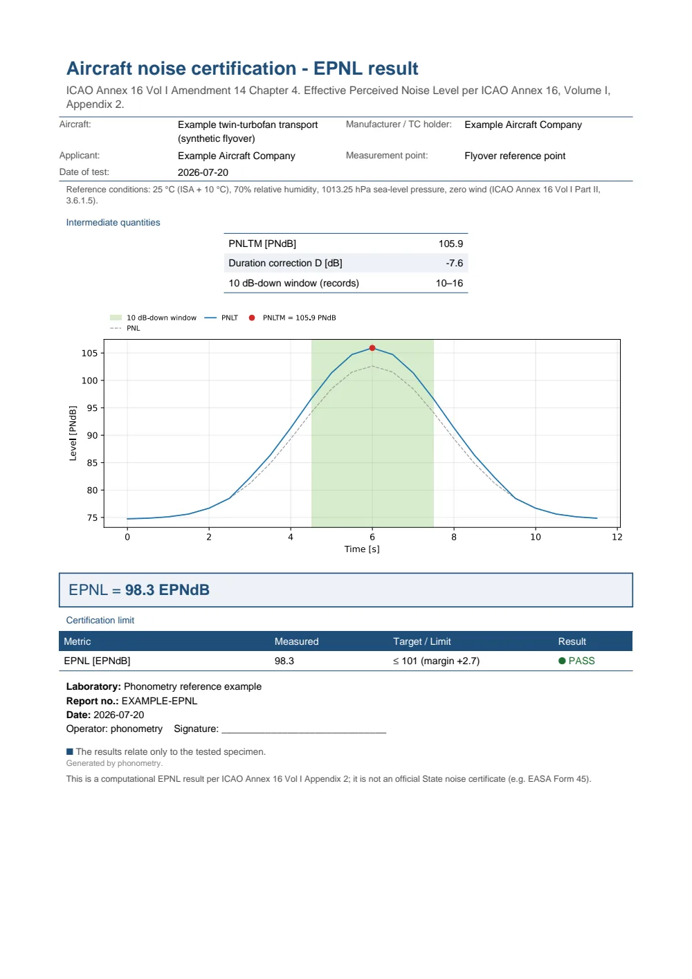
One-page aircraft-noise-certification fiche: a metadata header, a reference-conditions strip, a metrics table with the peak PNLTM and the duration correction D and the 10 dB-down record window, the full-width PNL/PNLT time-history plot with the marked PNLTM and the shaded integration window, the boxed EPNL = 98.3 EPNdB single-number result and a PASS verdict against a 101 EPNdB certification limit.
From a measured flyover to a certification level
Section titled “From a measured flyover to a certification level”What the section above computed is the EPNL of the flight as flown, on the day it was flown. A certification level is the same quantity transported to a fixed reference day (sea-level pressure of 1 013.25 hPa, 25 °C at sea level with the ICAO Standard Atmosphere lapse rate, 70 % relative humidity, zero wind, per Chapter 3 §3.6.1.5) and to a fixed reference flight path. Appendix 2 §8 is that transport, and it is the missing half of the chain.
In the simplified method (§8.3) each band of the spectrum is moved to the reference day by
which swaps the test-day absorption coefficient for the reference one over the measured path, re-absorbs over the corrected path length, and applies an inverse-square term for the change in path length (§8.3.2.1). The adjusted spectrum is re-run through the noy law and the tone correction, the bandsharing adjustment of the test day is added back, and the difference is one of four terms added to the measured EPNL:
(§8.3.6). handles a secondary peak within 2 dB of that overtakes the adjusted maximum (§8.3.3); is the change in duration from the path length and the ground speed (§8.3.4); and corrects for the difference between the propulsion operating parameters flown and those specified for the reference condition, from manufacturer sensitivity curves (§8.3.5). §8.2.3 fixes when the simplified method is not enough and the integrated method must be used instead: a flyover disagreement above 8 EPNdB, an approach disagreement above 4 EPNdB, or a result within 1 EPNdB of the Chapter 3 limit.
The library supplies the ingredients and not the bookkeeping. air_attenuation
and sae_band_attenuation below are exactly the and
of the first two terms, and the EPNL machinery re-runs an adjusted spectrum as
readily as a measured one; the flight-path geometry and the four
terms themselves are not implemented. Adjust first, then report: the
EPNL this page returns is a test-day value, and a requirement verdict is only
a certification verdict once §8 has been applied.
Measurement-system verification (IEC 61265)
Section titled “Measurement-system verification (IEC 61265)”verify_aircraft_noise_system checks measured performance against the
IEC 61265:1995 tolerances: the microphone directional-response limits (Table 1,
identical to Annex 16 Table A2-1) and the scalar frequency-response, linearity
and resolution limits.
The arguments are measured data, not settings. The outer key of directional
is a one-third-octave midband frequency in hertz; the inner key is the sound
incidence angle in degrees from the microphone’s principal axis; and the value
is the measured free-field sensitivity-level difference in decibels relative
to 0°, normal incidence, for sinusoidal waves in a free field. At 4 kHz the
limits are 0.5 / 1.0 / 2.0 / 2.5 / 2.5 dB at 30 / 60 / 90 / 120 / 150°, so the
example below passes with margin. That check matters because the aeroplane
sweeps through a wide range of incidence angles while the microphone stays
fixed, and the whole station is built around sound arriving within a few degrees
of grazing. frequency_response values are deviations in decibels from the
level at the calibration-check frequency, in the reference direction.
The data comes from an anechoic free-field turn of the microphone with its
windscreen fitted, or from an actuator response plus the supplier’s free-field
corrections; the electrical half comes from inserting a low-distortion sinusoid
within 5 dB of the calibration level and stepping it in 5 dB intervals, refined
to 1 dB around the ends of the linear range and the overload point. Run and
report the periodic test in a controlled environment (19-25 °C, 100-102 kPa,
40-70 % relative humidity) with a calibrator traceable to national standards.
Read report.passes as a verdict on data you supplied: a failed check
invalidates the certification data, it is not a correction to apply. Band-filter
conformance is a separate matter: Annex 16 §3.7.3 requires IEC 61260 class 1,
with class 2 admissible only if the certificating authority allows it, and the
library’s own filter verification is the place that is checked.
from phonometry import aircraft
report = aircraft.verify_aircraft_noise_system(    directional={4000.0: {30: 0.4, 60: 0.9, 90: 1.9, 120: 2.4, 150: 2.4}},    frequency_response={1000.0: 1.2},)print(report.passes, report.checks)
Atmospheric absorption (SAE ARP 5534)
Section titled “Atmospheric absorption (SAE ARP 5534)”Correcting a measured flyover to reference atmospheric conditions needs the
one-third-octave-band attenuation over the path. The pure-tone coefficient is
the ISO 9613-1 one (identical, per ARP 5534 §3.1) provided by air_attenuation;
sae_band_attenuation adds the SAE Method (ARP 5534 §3.2.2) mapping the
pure-tone mid-band path attenuation to the band
attenuation , consistent with the Exact Method well beyond the 50 dB
Approximate-Method limit.
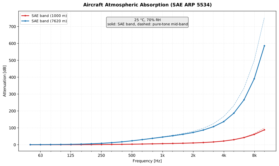
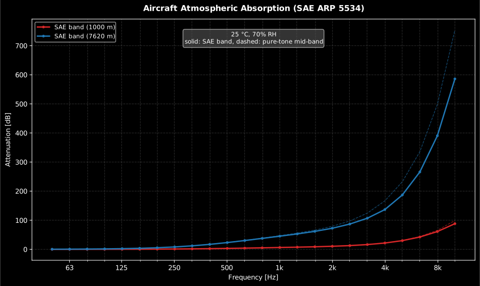
Solid is the band, dashed the pure tone at the band centre, and the two only coincide where the absorption is small. At 1 km the gap is 0.18 dB in the 4 kHz band and 10.78 dB at 10 kHz; at 7620 m it is 29.95 dB at 4 kHz and 167.97 dB at 10 kHz, against a mid-band value of 753.92 dB. Both are the same 25 °C, 70 % RH atmosphere: the difference is that a band keeps the energy of its low edge long after its centre frequency has gone.
A third-octave band is not a tone. The absorption coefficient rises steeply with frequency, so the low edge of a band is attenuated far less than its midband frequency, and as the path lengthens the surviving band energy is carried almost entirely by that lower half. The band attenuation therefore falls progressively behind the pure-tone value, which is what the two curves show: at 1 km they are indistinguishable below a few kilohertz and separate only at the top of the range, while at 7620 m the gap at high frequency is large. This is exactly the regime the older 50 dB-limited Approximate Method of ARP 866B could not follow. The consequence for §8 is direct: correcting a flyover to reference conditions with the pure-tone coefficient overstates the high-frequency correction, and with it the reference-day EPNL.
Show the code for this figure
import matplotlib.pyplot as pltimport numpy as npfrom phonometry import aircraft
freqs = 1000.0 * 10.0 ** (np.arange(-13, 11) / 10.0)   # 50 Hz-10 kHz thirdsfig, ax = plt.subplots()# solid: SAE band attenuation, dashed: pure-tone mid-bandfor s in (1000.0, 7620.0):    att = aircraft.sae_band_attenuation(        freqs, s, temperature_c=25.0, relative_humidity_percent=70.0    )    line, = ax.semilogx(att.frequencies, att.band_attenuation, marker="o",                        markersize=3, label=f"SAE band ({s:.0f} m)")    ax.semilogx(att.frequencies, att.midband_attenuation, "--", alpha=0.6,                color=line.get_color())ax.set(xlabel="Frequency [Hz]", ylabel="Attenuation [dB]",       title="Aircraft atmospheric absorption at 25 °C, 70% RH")ax.grid(True, which="both", alpha=0.3)ax.legend()plt.show()
import numpy as npfrom phonometry import aircraft
freqs = 1000.0 * 10.0 ** (np.arange(-13, 11) / 10.0) # 50 Hz–10 kHz thirdsatt = aircraft.sae_band_attenuation(freqs, path_length=7620.0, temperature_c=25.0, relative_humidity_percent=70.0)att.plot() # band vs pure-tone mid-band (needs matplotlib)The regression was fitted for roughly 6-32 °C and 20-95 % relative humidity (the 14 CFR Part 36 test window) and for path lengths up to 7620 m (25 000 ft). The function’s defaults (25 °C and 70 % RH) are the ARP 5534 reference point and the Annex 16 reference day. The mapping is reciprocal, so the same call serves both directions of the reference-condition adjustment: removing the test-day absorption from a measured record, and re-applying the reference-day absorption to it.
The certification chain ends here. Turning these aeroplanes into noise around an airport, the noise-power-distance tables, the per-segment corrections of a flight path and the ground contour of a single event, is the ECAC Doc 29 method of Airport noise.
What this guide covers
Section titled “What this guide covers”Covered
ICAO Annex 16, Vol. I, Appendix 2: perceived noisiness and PNL from Table A2-3 (
perceived_noisiness,perceived_noise_level), the slope- method tone correction (tone_correction, matching the ETM Vol. I Table 3-7 turbofan example) and the full EPNL chain (effective_perceived_noise_level, matching the ETM Vol. I Table 4-4 example). IEC 61265:1995 measurement-system tolerances viaverify_aircraft_noise_system. SAE ARP 5534 band atmospheric absorption viasae_band_attenuation.Not covered
The Appendix 2 §8 adjustment of a measured EPNL to reference conditions is not implemented, in either the simplified or the integrated form: the returned EPNL is the as-measured value, so adjust first and then report against a limit.
verify_aircraft_noise_systemchecks the IEC 61265:1995 tolerances, not the superseding 2018 edition. The ECAC Doc 29 airport-noise chain has moved to Airport noise.
References
Section titled “References”- International Civil Aviation Organization. (2017). Annex 16 to the Convention on International Civil Aviation: Environmental protection — Volume I: Aircraft noise (ICAO Annex 16, Vol. I, 8th ed.). The normative Appendix 2 EPNL procedure implemented by the noisiness, tone correction and EPNL sections.
- International Civil Aviation Organization. (2018). Environmental technical manual — Volume I: Procedures for the noise certification of aircraft (Doc 9501, 3rd ed.). The worked examples (Table 3-7 tone correction, Table 4-4 integrated-method EPNL) used as the numeric oracles.
- International Electrotechnical Commission. (1995). Electroacoustics — Instruments for measurement of aircraft noise — Performance requirements for systems to measure one-third-octave-band sound pressure levels in noise certification of transport-category aeroplanes (IEC 61265:1995). The measurement-system tolerances checked by the verifier. Since revised as IEC 61265:2018 (https://webstore.iec.ch/en/publication/32635); the 1995 edition is the implemented one.
- SAE International. (2012). Standard values of atmospheric absorption as a function of temperature and humidity (SAE ARP 866B, stabilized 2012). The predecessor SAE atmospheric-absorption practice, source of the 50 dB-limited Approximate Method the SAE Method is contrasted with.
- SAE International. (2013). Application of pure-tone atmospheric absorption losses to one-third octave-band data (SAE ARP 5534, reaffirmed 2021). The SAE-Method band attenuation of the atmospheric-absorption section, with the pure-tone coefficient from ISO 9613-1.