Benchmarking

The benchmark command measures RouterOS API operations against a real router. It is intended for development and capacity planning, not for normal deployments.

Command

Build and run the benchmark:

go run ./cmd/benchmark

The config path is optional and defaults to config/test.yaml:

go run ./cmd/benchmark config/test.yaml

The benchmark reads the MikroTik section from the selected YAML file, connects to RouterOS, then runs API-level operations.

What it measures

• Single IPv4 and IPv6 address-list adds/removes.
• Address-list find and list calls.
• Firewall rule create, find, and remove calls.
• Sequential IPv4 batch add/list/find/remove timings.

The benchmark uses documentation-prefix test addresses such as 198.51.100.0/24 and 2001:db8::/32, but it still writes to the configured RouterOS address lists and firewall menus.

Caution

Run benchmarks on a lab router or during a maintenance window. The command creates temporary firewall rules and address-list entries and then removes them.

Example output

Connected to: lab-router

=== SINGLE OPERATION BENCHMARKS (RouterOS API) ===
  Add single IPv4                         35ms  OK
  Find IPv4 (1 entry)                     12ms  OK
  Remove IPv4 by .id                      18ms  OK

=== BATCH ADD BENCHMARKS (sequential via API) ===
  Add 100 IPv4 (sequential)                4s  (40ms/ip, failures=0)

Use the numbers to compare RouterOS versions, hardware models, TLS vs plaintext API, and network latency.

For real bouncer startup performance, prefer the functional CAPI tests because reconciliation uses script-based bulk adds and pool-based removals, not only sequential API calls.

Real-world results

These figures come from the functional CAPI test suite (tests/functional/) run against a MikroTik RB5009, not from the single-operation cmd/benchmark tool above. See Architecture: Connection pool and Script-based bulk add for the mechanisms behind these numbers.

Scenario	Result
Cache-first optimistic add (address not yet on the router)	~1–3 ms per operation
Check-first add (list entries before adding, avoided by cache)	~400 ms per IP
Script-based bulk add vs. sequential API calls	~97× faster for large batches
Full RB5009 bulk-add, ~22,000 CAPI-origin entries	~29 s bulk, ~34 s from start

The gap between cache-first (~1-3 ms) and check-first (~400 ms) is why the in-memory address cache described in Architecture exists: it lets the bouncer skip the RouterOS list-then-add round trip for addresses it already knows about.

For CAPI-scale deployments (tens of thousands of entries), also see CAPI Blocklists and Performance Tuning for pool_size sizing guidance.

The full lifecycle, sampled every 100 ms

The chart below is a single continuous 70-second capture from the production RB5009, taken with a 10 Hz sampler reading /proc/stat on the router itself (see the note on method at the end of this page). It covers the three states an operator actually meets: the router idle with the bouncer stopped and the address list empty, the first reconciliation importing ~22,000 entries, and the quiet state that follows with the full list in place. CPU reads on the left axis, RAM on the right, and the dashed markers are taken from the bouncer’s own log timestamps. Each point is the mean of five 100 ms samples; the sub-second peaks reach 57% for single 100 ms slices during the import.

First reconciliation on an RB5009 holding 22,000 entries. Regenerated with go run ./cmd/perfmon plot from the committed dataset.

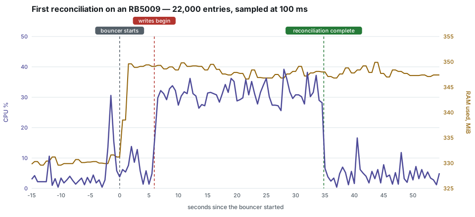
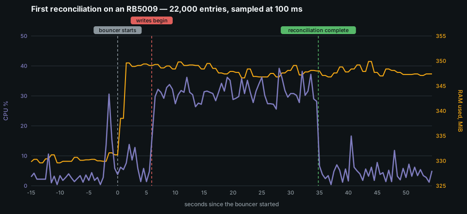
The import is the plateau: roughly 31% sustained for ~26 seconds, spread across all four cores with the connection pool rotating single-core peaks of 50–100%. RAM is the quiet part of the story, with one surprise in the timing: the ~19 MiB step lands at connection time, before a single entry is imported — and 22,000 entries later it has not moved again. Holding the list costs the router almost nothing; memory is not where this workload bites, CPU during list reads is. The idle stretch also shows the router’s own background blips — a real device is never a flat line.

Method note

The 100 ms series comes from a sampler container running on the router itself, reading the shared kernel’s /proc/stat and /proc/meminfo at 10 Hz and pushing batches straight to Loki — RouterOS’s own cpu-load updates only once per second, so scripts cannot see below that. The capture protocol: stop the bouncer, delete both address lists, let the router settle, then start the bouncer and record through the first reconciliation into steady state.

The whole instrumentation deploys with one command against any RouterOS device with the container package enabled:

go run ./cmd/perfmon install -router admin@192.168.88.1 -port 22 \
  -loki http://your-loki:3100

It cross-builds the sampler, packs the container image without needing Docker, creates the veth, NAT and firewall-list memberships idempotently, starts the container and verifies that samples reach Loki. uninstall removes exactly what it created; capture pulls any window as CSV; plot redraws the chart above from the committed dataset. Run any verb with -h for the full flag list.

Measuring against a live router

Two habits separate a number you can act on from one that misleads, and both were learned the expensive way while tuning this bouncer.

Interleave the arms. A router is not a quiet machine: it routes traffic, runs its own background work, and drifts over minutes. Measuring variant A for a while and then variant B for a while attributes that drift to the change. Alternate them instead — A, B, A, B — inside the same connection and the same minute, and compare paired samples. The first in-situ comparison of the proplist reduction ran as two separate windows and reported −2%; the interleaved run reported −11.2%, with every one of 48 pairs favouring the same side. Same code, same router; only the schedule differed.

Distrust a curve that is not monotonic. Sweeping the bulk chunk size once per value, in sequence, produced this:

chunk 50    6.926s
chunk 100   4.679s
chunk 250   9.760s     <- twice its neighbours on both sides
chunk 500   5.395s
chunk 1000  6.194s

No cost model produces that shape.

Report a spread, not a single number. The obvious repair — interleave the sizes across rounds and take the best time each — is still wrong, just less obviously. A minimum is a defensible estimator when noise is one-sided, but it throws away exactly the information that decides whether the comparison means anything. Re-run keeping every sample, the same sweep says:

chunk	median	mean	IQR
50	5.78 s	6.86 s	1.76 s
100	5.06 s	5.31 s	0.22 s
250	5.31 s	6.39 s	2.47 s
500	5.50 s	5.77 s	0.84 s
1000	4.36 s	5.75 s	2.55 s

The spread within a single chunk size reaches 2.55 s, while the gap between the best and worst size is 1.43 s. The noise on one arm is larger than the difference between arms, so the sweep resolves nothing — and sure enough, which size “wins” depends on the estimator: median and minimum pick 1,000, the mean picks 100. Reporting only the best of three rounds would have hidden all of that behind a clean-looking table.

The conclusion survived, because it never rested on the ranking: inserting a row dominates, so no chunk size in this range moves the import measurably. But the first write-up of it stated a two-term cost model to two significant figures that the data does not support.

A useful reflex: before believing a result, ask what else changed between the two measurements. Usually it is time.

Safety checklist

• Confirm the target is a lab router.
• Use dedicated test address lists when possible.
• Keep command_timeout high enough for slow devices.
• Check the router after interruption and remove any benchmark-* comments if a run is stopped midway.