Source: https://jmrplens.github.io/phonometry/signals/filters/filter-banks/ # Filter Banks phonometry supports several filter types, each with its own transfer function characteristic. Butterworth, Chebyshev II and Bessel place their **−3 dB points on the ANSI S1.11 band edges**, so their band levels are directly comparable. The two equiripple designs (Chebyshev I, Elliptic) do not: they take those edges as the *ripple* edge instead, which widens the band and biases every band level by a fixed few tenths of a decibel — see section 1. ## 1. Fractional octave bands: the math IEC 61260-1:2014 builds every band from the base-10 octave ratio $G = 10^{3/10} \approx 1.99526$ (so "one octave" is *not* exactly 2). For band fraction $1/b$, the mid frequencies and band edges follow (5.2-5.5): $$ f_\mathrm{m} = 1000 \cdot G^{x/b} \quad (b\ \text{odd}), \qquad f_1 = f_\mathrm{m} G^{-1/2b}, \quad f_2 = f_\mathrm{m} G^{+1/2b} $$ so every 1/3-octave band spans $G^{1/3} \approx 1.2589 \approx 10^{1/10}$: ten bands per decade, which is why the nominal frequencies (25, 31.5, 40 …) repeat scaled by 10. phonometry designs each band as an SOS cascade on those edges, but only three of the five architectures put their −3 dB points on $f_1$ and $f_2$. Butterworth's SciPy design frequency *is* its −3 dB point; Chebyshev II is designed through its stopband edges, mapped back from the band edges analytically, and Bessel is normalized with `norm="mag"` — both corrections exist so that their −3 dB points land on the edges too. Chebyshev I and Elliptic are handed the band edges directly, and SciPy reads them as the *equiripple passband* edge: at the default `ripple=0.1` the response there is −0.10 dB rather than −3 dB, the band is effectively wider, and every band level carries a systematic offset — median +0.33 dB (`cheby1`) and +0.25 dB (`ellip`) against Butterworth over a one-third-octave bank analysing 20 s of white noise. That offset is a *bias*, not scatter: it does not shrink with averaging time and it moves every band at once, so choose one architecture per campaign and never mix architectures inside one spectrum. ### Poles, zeros and stability A digital band-pass filter is a constellation of poles and zeros in the z-plane: zeros at or near DC and Nyquist pin the response down far from the band (to the stopband floor, for equiripple designs), and the poles cluster just inside the unit circle at the angles $\omega = 2\pi f / f_\mathrm{s}$ the passband spans. Two intuitions follow. First, selectivity is proximity: the closer the poles sit to the unit circle, the sharper the band and the longer the filter rings (the group-delay peaks of section 4 are that ringing, measured). Second, stability is a margin, not a property of the architecture: an IIR filter is stable only while every pole stays strictly inside the unit circle, and a narrow band at a high sample rate pushes the poles outward (pole radius $\approx 1 - \pi B / f_\mathrm{s}$ for bandwidth $B$) and squeezes them together, until double-precision coefficients can no longer represent their positions accurately. Second-order sections (SOS) defuse half of the problem: each pole pair keeps its own coefficients, so rounding errors stay local instead of compounding through one high-order polynomial. The other half, the tiny $B / f_\mathrm{s}$ ratio itself, is what decimation fixes. 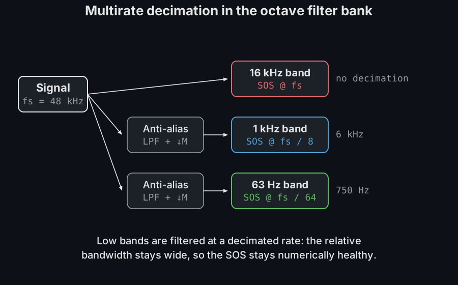### Multirate decimation A 25 Hz one-third-octave band at 48 kHz spans about 5.8 Hz, 0.024 % of Nyquist, with coefficients so stiff they go numerically unstable. The bank avoids that by filtering low bands at a decimated rate: Decimating by $M$ rescales the problem: the same 5.8 Hz bandwidth becomes $M$ times larger relative to the new Nyquist, the pole radius pulls away from the unit circle, and the SOS coefficients return to a well-conditioned range. The price is bookkeeping the bank pays internally: an anti-alias low-pass must run before every decimation stage, because a component above the new Nyquist that folds down lands *inside* the low bands being measured, and no later filter can remove it. ### Aliasing pitfalls The bank protects its own decimation stages, but it can only analyze what the capture chain delivered: - **Fold-down at the ADC.** Energy above $f_\mathrm{s}/2$ that reaches the converter without an analog anti-alias filter folds into the analysis range and is indistinguishable from real in-band sound. Sound cards filter this internally; custom instrumentation chains may not. - **Cheap resampling.** Converting a 44.1 kHz recording to 48 kHz with a low-quality resampler leaves images that bias the highest bands. Use a polyphase resampler (`scipy.signal.resample_poly`) or, simpler, analyze at the native rate: every phonometry function takes `fs` directly. - **Bands near Nyquist.** A band whose upper edge approaches $f_\mathrm{s}/2$ cannot realize its design response: the bilinear transform compresses the frequency axis there (the same effect the weighting filters counter with `high_accuracy`). Keep the top band edge comfortably below Nyquist or raise `fs`, and let `verify_filter_class` report how much margin is left. ### How long must the record be? A band level is not read off a signal, it is *estimated* from it, and the narrower the band the longer that takes. The bandwidth of a $1/b$-octave band is $B = f_\mathrm{m}\,(G^{1/2b} - G^{-1/2b})$ — $0.231\,f_\mathrm{m}$ for one-third octaves — and two consequences follow. The filter has to **settle**: a band rings for a few times $1/B$, so that much of the front of the record is transient rather than level (about a second in the 12.5 Hz band, twelve milliseconds at 1 kHz). And the estimate carries a **random error** of about $4.34/\sqrt{BT}$ dB on noise-like sound, so a 0.4 dB standard deviation needs $BT = 100$: 35 s of record for the 12.5 Hz band, 3.5 s for 125 Hz, 0.4 s for 1 kHz. The rule is one line: the lowest band you intend to report sets the record length for the whole bank. Analysing a 1 s clip down to 12.5 Hz and reporting the result to one decimal is not a measurement of that band, and neither `octave_filter` nor `OctaveFilterBank` warns you. The band mathematics above is shared by every architecture. How the architectures actually differ, the comparison at the −3 dB crossover, the full 1/1 and 1/3 octave response gallery and the usage examples per architecture, up to the Linkwitz-Riley crossover, is [Filter Architecture Gallery](https://jmrplens.github.io/phonometry/signals/filters/filter-gallery/). ## 2. `octave_filter()` / `OctaveFilterBank` parameters The advanced options travel in four small frozen dataclasses, so the four everyday arguments stay first: `FilterDesign` (`design`), `LevelCalibration` (`calibration`), `BlockProcessing` (`block_processing`) and `ResponsePlot` (`response_plot`). The table names each option by its bundle. | Parameter | Type | Units | Range / default | Notes | | :--- | :--- | :--- | :--- | :--- | | `x` | 1D or 2D array | digital units | non-empty | 2D is `[channels, samples]` | | `fs` | int | Hz | > 0 | | | `fraction` | int | — | default `1`; common `3`; any $b \ge 1$ | Bands per octave = $b$ | | `order` | int | — | default `6` | SOS order per band | | `limits` | list `[lo, hi]` | Hz | default `[12, 20000]` | Analysis range | | `design.filter_type` | str | — | `'butter'` (default), `'cheby1'`, `'cheby2'`, `'ellip'`, `'bessel'` | See the [Filter Architecture Gallery](https://jmrplens.github.io/phonometry/signals/filters/filter-gallery/) | | `design.ripple` / `design.attenuation` | float | dB | `ripple` default `0.1`; `attenuation` default `72.0` | Passband ripple / stopband attenuation (cheby/ellip); `cheby2` needs `attenuation` $\ge 70$ for class 1, since scipy pins its equiripple floor at exactly this value | | `design.resample` | bool | — | default `True` | Filter each band on a decimated rate (multirate) | | `response_plot.show` | bool | — | default `False` | Plot the bank response (needs matplotlib) | | `sigbands` | bool | — | default `False` | Also return the per-band time signals | | `mode` | str | — | `'rms'` (default) or `'peak'` | Per-band statistic returned | | `nominal` | bool | — | default `False` | Return nominal band labels (e.g. `1000`) instead of exact centre frequencies | | `detrend` | bool | — | default `True` | Remove each band's DC offset before the level (improves low-frequency accuracy) | | `calibration.factor` | float | — | default `1.0` | Scales the input to pascals (see the Calibration guide) | | `calibration.dbfs` | bool | — | default `False` | Reference levels to digital full scale instead of 20 µPa | | `response_plot.file` | str or `None` | — | default `None` | Save the bank-response plot to this path | | `zero_phase` | bool | — | default `False` | Forward-backward filtering (offline) | | `block_processing.stateful` / `.steady_ic` (class) | bool | — | default `False` | Streaming state; see [Block Processing](https://jmrplens.github.io/phonometry/signals/filters/block-processing/) | `mode` has exactly two values. `'rms'` reports the energy-mean level of the band over the whole record, which is what every standard means by "band level". `'peak'` reports $20\log_{10}$ of the largest absolute sample inside the band: an instantaneous, band-limited, unweighted peak — not the C-weighted $L_\mathrm{Cpeak}$ of the [Levels](https://jmrplens.github.io/phonometry/signals/levels/levels/) guide — and on impulsive signals it is dominated by the filter's own ringing. There is no `'sum'` mode: a total across bands is an energy sum the caller performs, `10*np.log10(np.sum(10**(spl/10)))`, never an arithmetic mean of decibels. `verify_filter_class(bank)` checks the designed bank against the IEC 61260-1 Table 1 acceptance limits and reports the class (`1`, `2` or `None` if outside both) with per-band margins. ## 3. Parametric EQ (`ParametricEQ`) Biquad equalizer sections per the **RBJ Audio EQ Cookbook** (Bristow-Johnson): peaking (bell), low/high shelf, low/high-pass, band-pass (constant 0 dB peak or constant skirt gain), notch and all-pass, each parameterized by `fs`, `f0`, `gain_db` and one of `q`, `bw` (bandwidth in octaves) or `slope` exactly as the cookbook defines them. Sections cascade as a numerically robust SOS chain, and the design is closed-form exact: a peaking section passes exactly `gain_db` at `f0` and exactly 0 dB at DC and Nyquist, shelves land exactly on `gain_db` at their shelved end, and the all-pass has unit magnitude everywhere (only the phase turns). ```python import numpy as np from phonometry import EQSection, ParametricEQ fs = 48000 rng = np.random.default_rng(1) x = rng.standard_normal(fs) # one second of noise eq = ParametricEQ(fs, [ EQSection("lowshelf", 100.0, gain_db=4.0), EQSection("peaking", 1000.0, gain_db=-6.0, bw=1.0), # one-octave cut EQSection("highshelf", 8000.0, gain_db=3.0), ]) y = eq.filter(x) # apply the cascade res = eq.response() # frozen result carrying the SOS cascade axes = res.plot() # magnitude + phase of the cascade ``` For block processing pass `stateful=True` (the same convention as `WeightingFilter`); the one-shot helper is `parametric_eq(x, fs, sections)`.

Show the code for this figure

```python import matplotlib.pyplot as plt from phonometry import EQSection, ParametricEQ fs = 48000 family = [ EQSection("peaking", 1000.0, gain_db=6.0, q=1.4), EQSection("lowshelf", 125.0, gain_db=6.0), EQSection("highshelf", 4000.0, gain_db=-6.0), EQSection("lowpass", 10000.0), EQSection("highpass", 50.0), EQSection("bandpass", 500.0, q=2.0), EQSection("notch", 2000.0, q=6.0), ] fig, ax = plt.subplots(figsize=(10, 6)) for section in family: res = ParametricEQ(fs, [section]).response(f_min=20.0, f_max=20000.0) ax.semilogx(res.frequencies, res.magnitude_db, label=f"{section.filter_type} @ {section.f0:g} Hz") ax.set(xlim=(20, 20000), ylim=(-27, 9), xlabel="Frequency [Hz]", ylabel="Magnitude [dB]") ax.grid(True, which="both", alpha=0.3) ax.legend(loc="lower center", ncols=2, fontsize=9) plt.show() ```

Everything above is design. Proving that a designed bank meets a performance class of IEC 61260-1, band by band and with its margin in decibels, is [Filter class verification](https://jmrplens.github.io/phonometry/signals/filters/filter-compliance/): the Table 1 acceptance mask, the stricter class 0 of the withdrawn 1995 edition, what a class buys in a measurement, and the accredited compliance fiche. ## 4. Signal Decomposition and Stability By setting `sigbands=True`, you can retrieve the time-domain components of each band. This allows for advanced analysis or comparing how different architectures (e.g., Butterworth vs Chebyshev) affect the signal phase and transient response. ```python import numpy as np from phonometry import filters # 1. Generate a signal (Sum of 250Hz and 1000Hz) fs = 48000 t = np.linspace(0, 0.5, int(fs * 0.5), endpoint=False) y = np.sin(2 * np.pi * 250 * t) + np.sin(2 * np.pi * 1000 * t) # 2. Compare architectures (Butterworth vs Chebyshev II) spl_b, freq, xb_butter = filters.octave_filter( y, fs=fs, fraction=1, sigbands=True, design=filters.FilterDesign(filter_type='butter')) spl_c2, _, xb_cheby2 = filters.octave_filter( y, fs=fs, fraction=1, sigbands=True, design=filters.FilterDesign(filter_type='cheby2')) # 'xb_butter' and 'xb_cheby2' contain the time-domain signals per band ``` *The plot compares the **Butterworth** (solid blue) and **Chebyshev II** (dashed red) responses. The bottom plot shows the **Impulse Response**, highlighting the differences in stability and transient decay.*

Show the code for this figure

```python import matplotlib.pyplot as plt import numpy as np from phonometry import filters fs = 48000 t = np.linspace(0, 0.5, int(fs * 0.5), endpoint=False) y = np.sin(2 * np.pi * 250 * t) + np.sin(2 * np.pi * 1000 * t) bank_b = filters.OctaveFilterBank(fs=fs, fraction=1, order=6, limits=[100.0, 2000.0]) bank_c = filters.OctaveFilterBank(fs=fs, fraction=1, order=6, limits=[100.0, 2000.0], design=filters.FilterDesign(filter_type="cheby2")) _, freq, xb_butter = bank_b.filter(y, sigbands=True) _, _, xb_cheby2 = bank_c.filter(y, sigbands=True) fig, axes = plt.subplots(len(freq), 1, figsize=(9, 2 * len(freq)), sharex=True) for ax, fc, xb, xc in zip(axes, freq, xb_butter, xb_cheby2): ax.plot(t, xb, label="Butterworth") ax.plot(t, xc, "--", label="Chebyshev II") ax.set_title(f"{fc:.0f} Hz band") ax.set_xlim(0, 0.04) axes[0].legend() axes[-1].set_xlabel("Time [s]") plt.tight_layout() plt.show() ```

> [!NOTE] > **Why do the signals look shifted in time?** > Digital IIR filters (like Butterworth or Chebyshev) have **non-linear phase > responses**, which results in frequency-dependent **Group Delay**. In the 250 Hz > band, you can see that the Chebyshev II filter has a different propagation delay > compared to the Butterworth filter. This is a normal physical property of these > architectures: more aggressive frequency roll-offs usually come at the cost of > higher group delay and phase distortion. ### Group delay, quantified The group delay $\tau_\mathrm{g}(\omega) = -\frac{d\phi(\omega)}{d\omega}$ of the 1 kHz octave band shows the trade-off directly: Bessel stays nearly flat across the passband (transient shapes survive), while Chebyshev I and Elliptic pay for their steep roll-off with strong delay peaks at the band edges.

Show the code for this figure

```python import matplotlib.pyplot as plt import numpy as np from scipy.signal import group_delay from phonometry import filters fs = 48000 w = np.logspace(np.log10(500), np.log10(2000), 1024) fig, ax = plt.subplots(figsize=(9, 5)) for ftype in ("butter", "cheby1", "cheby2", "ellip", "bessel"): bank = filters.OctaveFilterBank(fs, fraction=1, order=6, limits=[800, 1200], design=filters.FilterDesign(filter_type=ftype)) idx = int(np.argmin(np.abs(np.array(bank.freq) - 1000))) fsd = fs / bank.factor[idx] # Group delay of an SOS cascade = sum of the sections' group delays gd = sum(group_delay((sec[:3], sec[3:]), w=w, fs=fsd)[1] for sec in bank.sos[idx]) ax.semilogx(w, gd / fsd * 1000, label=ftype) ax.set(xlim=(500, 2000), xlabel="Frequency [Hz]", ylabel="Group delay [ms]") ax.grid(True, which="both", alpha=0.3) ax.legend() plt.show() ```

## 5. Zero-phase filtering For offline analysis you can eliminate group delay entirely: `OctaveFilterBank.filter(…, zero_phase=True)` filters each band forward-backward (`scipy.signal.sosfiltfilt`), keeping band signals time-aligned with the input. It is a per-call option on the bank, not an argument of the one-shot `octave_filter()`, which rejects it with a `TypeError`. The effective attenuation doubles and the effective passband narrows, lowering the measured broadband band level by ~0.2 to 0.3 dB per band (a pure in-band tone is unaffected); prefer forward filtering when the absolute band SPL must match single-pass conventions, and reserve zero-phase for when the temporal envelope matters (e.g. reverberation decay). The option is incompatible with stateful (block) processing. ```python import numpy as np from phonometry import filters fs = 48000 t = np.linspace(0, 0.5, int(fs * 0.5), endpoint=False) y = np.sin(2 * np.pi * 250 * t) + np.sin(2 * np.pi * 1000 * t) bank = filters.OctaveFilterBank(fs=48000, fraction=3) spl, freq, xb = bank.filter(y, sigbands=True, zero_phase=True) ``` *Causal filtering delays the burst by the filter's group delay; zero-phase filtering keeps it aligned with the input.*

Show the code for this figure

```python import matplotlib.pyplot as plt import numpy as np from phonometry import filters fs = 48000 t = np.linspace(0, 0.15, int(fs * 0.15), endpoint=False) x = np.zeros_like(t) # 250 Hz tone burst mid-frame start, end = int(0.05 * fs), int(0.10 * fs) x[start:end] = np.sin(2 * np.pi * 250 * t[start:end]) * np.hanning(end - start) bank = filters.OctaveFilterBank(fs=fs, fraction=1, order=6, limits=[200.0, 300.0]) _, _, fwd = bank.filter(x, sigbands=True, calculate_level=False) _, _, zp = bank.filter(x, sigbands=True, calculate_level=False, zero_phase=True) fig, ax = plt.subplots(figsize=(9, 4.5)) ax.plot(t, x, color="gray", alpha=0.5, label="Input burst (250 Hz)") ax.plot(t, fwd[0], label="Causal (group delay)") ax.plot(t, zp[0], "--", label="zero_phase=True (aligned)") ax.set(xlabel="Time [s]", ylabel="Amplitude") ax.legend() plt.show() ```

## Quick answers ### How are fractional-octave centre frequencies and band edges defined? IEC 61260-1:2014 (clauses 5.2-5.5) builds every band from the base-10 octave ratio $G = 10^{3/10} \approx 1.99526$, so one octave is not exactly 2. Mid frequencies follow $f_\mathrm{m} = 1000 \cdot G^{x/b}$ (for odd $b$) and the edges are $f_1 = f_\mathrm{m} G^{-1/2b}$ and $f_2 = f_\mathrm{m} G^{+1/2b}$; every one-third-octave band spans $G^{1/3} \approx 1.2589$, ten bands per decade. ## See also - [Filter Architecture Gallery](https://jmrplens.github.io/phonometry/signals/filters/filter-gallery/): the five architectures compared at the band edges, the full response gallery and per-architecture usage, with the Linkwitz-Riley crossover. - [Filter Class Verification (IEC 61260-1)](https://jmrplens.github.io/phonometry/signals/filters/filter-compliance/): the Table 1 acceptance mask, class 0 and the compliance fiche of the banks designed here. - API reference: [`phonometry`](https://jmrplens.github.io/phonometry/reference/api/filters/phonometry/), [`filters.core`](https://jmrplens.github.io/phonometry/reference/api/filters/core/) and [`filters.weighting`](https://jmrplens.github.io/phonometry/reference/api/filters/weighting/). - Theory: [Octave Band Frequencies](https://jmrplens.github.io/phonometry/reference/theory/signal-analysis/#octave-band-frequencies-ansi-s111--iec-61260): where the base-10 midband grid and the band edges come from, and why the bank is designed on them rather than on nominal labels. ## References - International Electrotechnical Commission. (2014). *Electroacoustics — Octave-band and fractional-octave-band filters — Part 1: Specifications* (IEC 61260-1:2014). [IEC webstore](https://webstore.iec.ch/en/publication/5063). The band-edge mathematics of section 1 and the nominal band labels behind every bank designed here. - Oppenheim, A. V., & Schafer, R. W. (2010). *Discrete-time signal processing* (3rd ed.). Pearson. ISBN 978-0-13-198842-2. [Open Library record](https://openlibrary.org/isbn/9780131988422). The pole-zero, stability and multirate theory condensed in section 1: SOS cascades, the bilinear transform and decimation. - Bristow-Johnson, R. *Audio EQ Cookbook*. Republished as a W3C Working Group Note (ed. R. Toy), 8 June 2021. [w3.org/TR/audio-eq-cookbook](https://www.w3.org/TR/audio-eq-cookbook/). The biquad coefficient recipes and the Q / bandwidth / shelf-slope parameterization behind `ParametricEQ` (section 3). - Smith, J. O. *Introduction to digital filters with audio applications* (online book). Center for Computer Research in Music and Acoustics (CCRMA), Stanford University. [ccrma.stanford.edu/~jos/filters](https://ccrma.stanford.edu/~jos/filters/). A free companion treatment of digital-filter design and analysis, from pole-zero geometry to filter stability. ## Standards IEC 61260-1:2014, *Electroacoustics — Octave-band and fractional-octave-band filters — Part 1: Specifications* — the base-10 mid frequencies and band edges of §1 (5.2-5.5) and the nominal band labels; its Table 1 class acceptance limits are verified in [Filter class verification](https://jmrplens.github.io/phonometry/signals/filters/filter-compliance/). ANSI S1.11-2004, *Octave-Band and Fractional-Octave-Band … Filters*: the band-edge convention on which every bank places its −3 dB points. ISO 266: the preferred-frequency series behind the nominal band labels reported by `nominal_frequencies`.