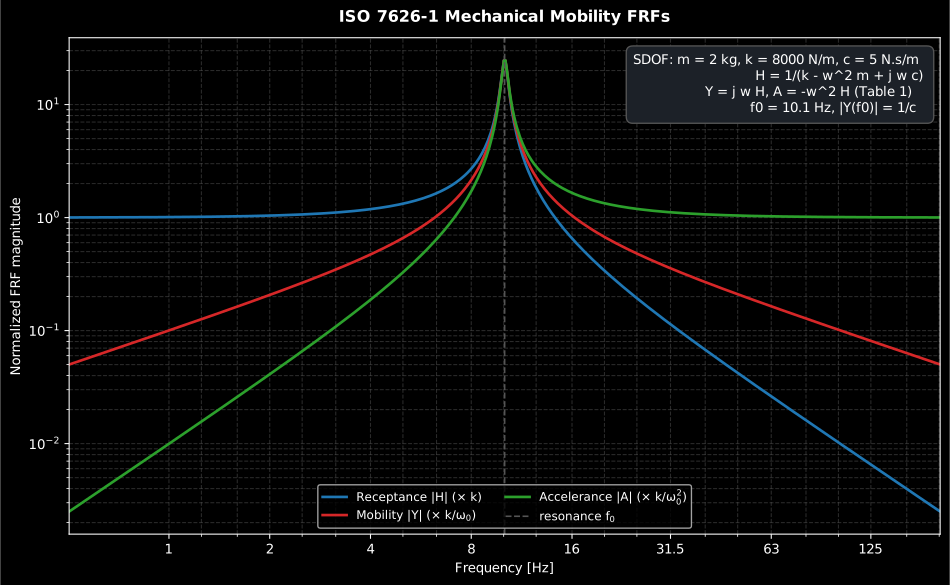
Source: https://jmrplens.github.io/phonometry/reference/api/vibration/mechanical-mobility/ # Mechanical mobility and the FRF family (ISO 7626-1) Mechanical **mobility** is the complex ratio of a velocity response to the force that produces it, `Y = v/F`. It is one member of a family of motion-per-force **frequency-response functions** (FRFs): which one is used depends only on whether the motion is a displacement, a velocity or an acceleration, and each has a force-per-motion reciprocal. **ISO 7626-1:2011** (*Mechanical vibration and shock — Experimental determination of mechanical mobility — Part 1: Basic terms and definitions, and transducer specifications*) defines the whole family (Table 1, with the 3.1.2 mobility definition), and the classic closed-form single-degree-of-freedom (SDOF) resonator serves as the reference for those definitions. **ISO 7626-2:2015** adds the measurement side: FRF estimation from measured signals and its acceptance criteria. This FRF backbone underpins the structure-borne source and transmission standards: ISO 9611, ISO 10846, EN 15657 and EN 12354-5.

Show the code for this figure

```python import matplotlib.pyplot as plt import numpy as np from phonometry import vibration m, k, c = 2.0, 8000.0, 5.0 f = np.logspace(np.log10(0.5), np.log10(200.0), 500) w = 2.0 * np.pi * f h = vibration.sdof_receptance(f, m, k, c) for label, frf in (("receptance |H|", np.abs(h)), ("mobility |Y|", np.abs(1j * w * h)), ("accelerance |A|", np.abs(-(w**2) * h))): plt.loglog(f, frf / frf.max(), label=label) plt.axvline(vibration.resonance_frequency(m, k), ls="--", color="0.6") plt.xlabel("Frequency [Hz]"); plt.ylabel("Normalized magnitude") plt.legend(); plt.show() ```

## 1. The frequency-response-function family (Table 1) For a harmonic motion `x·e^{jωt}` the velocity is `jω·x` and the acceleration `−ω²·x`, so all three motion-per-force FRFs follow from the receptance `H` by a power of `jω`, and each has a force-per-motion reciprocal: | Motion | FRF (motion / force) | Unit | Reciprocal (force / motion) | Unit | |---|---|---|---|---| | displacement | receptance `H = x/F` | m/N | dynamic stiffness `1/H` | N/m | | velocity | mobility `Y = jω·H` | m/(N·s) | impedance `1/Y` | N·s/m | | acceleration | accelerance `A = −ω²·H` | 1/kg | apparent mass `1/A` | kg | `convert_frf` moves between any two of the six FRFs, pivoting through the receptance. A **driving-point** FRF has the response and force at the same point (`i = j`); a **transfer** FRF has them at different points. Note that the force-per-motion kinds are element-wise reciprocals: the *free* quantities of ISO 7626-1, 3.1.4; the *blocked* matrix quantities of Table 1 do not invert element-wise for multi-coordinate systems (Table 1 also names `F/a` the "effective mass", the quantity called apparent mass here). ```python from phonometry import vibration # A mobility of 2e-3 m/(N.s) at 80 Hz, expressed as the other FRFs: Y = 2e-3 print(round(abs(vibration.convert_frf(Y, 80.0, "mobility", "impedance")), 1)) # 500.0 N.s/m print(f"{abs(vibration.convert_frf(Y, 80.0, 'mobility', 'accelerance')):.3f}") # 1.005 1/kg ``` The choice between the three motion FRFs is one of convenience, not physics: they carry the same information and `convert_frf` moves between them exactly. Accelerance is what an accelerometer-based measurement delivers directly; mobility is the natural currency of the structure-borne power standards (power is force times velocity, so `P = ½·Re{Y}·|F|²` at a contact); the reciprocals appear whenever a source is described by what it imposes rather than by how it responds. Reading a driving-point mobility plot is a structural diagnosis in itself: below a resonance the magnitude climbs proportionally to frequency along a **stiffness line** (`|Y| ≈ ω/k`), above it the magnitude falls along a **mass line** (`|Y| ≈ 1/(ωm)`), and the height of the peak between them reflects the damping: it equals `1/c` for the isolated viscously damped resonator of the next section, while on real structures with overlapping modes damping is instead estimated by modal fitting or from the half-power bandwidth. ## 2. The SDOF reference resonator (closed form) The canonical closed-form reference, expressed in the Table 1 / 3.1.2 FRF taxonomy, is a mass `m`, viscous damping `c` and stiffness `k`, whose receptance is $$ H(\omega) = \frac{1}{k - \omega^2 m + j\,\omega c}, \qquad \omega_0 = \sqrt{k/m}. $$ At the resonance `ω0` the driving-point mobility is **purely real** and equal to `1/c` (the mobility peak measures the damping) while the static receptance (`ω → 0`) is the compliance `1/k`: ```python import numpy as np from phonometry import vibration m, k, c = 2.0, 8000.0, 5.0 f0 = vibration.resonance_frequency(m, k) # 10.07 Hz y0 = complex(vibration.sdof_mobility(f0, m, k, c)) print(round(y0.real, 4), round(y0.imag, 6)) # 0.2 0.0 -> |Y(f0)| = 1/c print(round(complex(vibration.sdof_receptance(1e-6, m, k, c)).real, 7)) # 0.000125 = 1/k ``` ## 3. Measured FRFs and their acceptance criteria (ISO 7626-2) In the usual ISO 7626-2 arrangement the structure hangs on a suspension soft enough that its rigid-body modes fall well below the first elastic resonance (the standard admits freely suspended or grounded structures; clause 5 asks for a support representative of the intended application), an exciter drives one point through an **impedance head** (a transducer stack measuring force and acceleration at the same point, which is what gives the attached-exciter setup its driving-point FRF), and accelerometers pick up the response elsewhere for the transfer FRFs. ISO 7626-5 covers the alternative of impact excitation with an exciter that is not attached to the structure, in practice usually an instrumented hammer: it trades the attached exciter's controlled spectrum for speed, with an excitation spectrum set by the impactor mass and tip stiffness. Processing measured random-excitation records per ISO 7626-2, 8.1.3 (the H1 estimator `Ĥ = G(response, force)/G(force, force)`) and the ordinary coherence `γ² = |Gxy|²/(Gxx·Gyy)` used for its data-quality checks are the library's existing spectral estimators [`transfer_function` and `coherence`](https://jmrplens.github.io/phonometry/guides/electroacoustics/) (H1 is their default). On top of them, two ISO 7626-2 acceptance criteria are provided: * **Operational rigid-mass calibration (7.5.2).** The measured FRF of a freely suspended rigid block of known mass must agree within ±5 % with `|A| = 1/m` (accelerance) or `|Y| = 1/(2πf·m)` (mobility). * **Random error (Annex A + 8.1.3).** Enough spectra must be averaged that the normalized random error `ε = √((1−γ²)/(2nγ²))` at each resonance of a driving-point mobility is below 5 %. ```python import numpy as np from phonometry import vibration # A 10 kg calibration block: |A| must be 1/m = 0.100 1/kg at every frequency. f = np.array([20.0, 100.0, 500.0]) res = vibration.rigid_mass_calibration_check([0.100, 0.102, 0.097], f, mass=10.0) print(res.passed, res.within_tolerance.tolist()) # True [True, True, True] # The Annex A example: coherence 0.8 needs about 75 averages for < 5 %. print(round(float(vibration.random_error_percent(0.8, 75)), 2)) # 4.08 % ``` The calibration check returns a `RigidMassCalibrationResult` carrying the per-frequency deviation and pass flags, and a `.plot()`: the measured FRF magnitude against the rigid-mass line with its ±5 % tolerance band (upper panel) and the relative deviation against the same band (lower panel, where a few-percent tolerance is actually readable). A calibration that drifts out of the band towards a few kHz points at a transducer or attachment-compliance error, exactly what the check is meant to catch: ```python import numpy as np from phonometry import vibration m = 10.0 # calibration block mass f = np.logspace(np.log10(20.0), np.log10(5000.0), 400) drift = 0.05 * (f / 2500.0) ** 2 # high-frequency drift measured = (1.0 / m) * (1.0 + 0.015 * np.sin(2 * np.pi * np.log10(f)) + drift) res = vibration.rigid_mass_calibration_check(measured, f, mass=m) print(res.passed) # False (drift exceeds 5 %) res.plot() ```

Show the code for this figure

```python import matplotlib.pyplot as plt import numpy as np from phonometry import vibration m = 10.0 f = np.logspace(np.log10(20.0), np.log10(5000.0), 400) drift = 0.05 * (f / 2500.0) ** 2 measured = (1.0 / m) * (1.0 + 0.015 * np.sin(2 * np.pi * np.log10(f)) + drift) res = vibration.rigid_mass_calibration_check(measured, f, mass=m) bad = ~res.within_tolerance fig, (top, bot) = plt.subplots(2, 1, sharex=True, figsize=(10, 7), gridspec_kw={"height_ratios": [1.5, 1.0]}) top.fill_between(f, res.expected * 0.95, res.expected * 1.05, color="C1", alpha=0.15, label="±5 % tolerance band") top.semilogx(f, res.expected, "--", color="C1", label="expected |A| = 1/m") top.semilogx(f, res.measured, color="C0", label="within tolerance") top.semilogx(f[bad], res.measured[bad], "o", color="C1", label="out of tolerance") top.set_ylabel("Accelerance |A| [1/kg]"); top.legend() bot.axhspan(-5.0, 5.0, color="C1", alpha=0.15) bot.semilogx(f, 100.0 * res.deviation, color="C0") bot.semilogx(f[bad], 100.0 * res.deviation[bad], "o", color="C1") bot.set_xlabel("Frequency [Hz]"); bot.set_ylabel("Deviation [%]") plt.show() ```

## 4. The `MobilityResult` bundle `sdof_mobility_result` bundles the FRF over frequency into a `MobilityResult`, which exposes `.magnitude`, `.phase`, `.to(target)` (any Table-1 kind) and a `.plot()` of `|Y(f)|` with the resonance marked: ```python import numpy as np from phonometry import vibration f = np.logspace(np.log10(0.5), np.log10(200.0), 400) res = vibration.sdof_mobility_result(f, mass=2.0, stiffness=8000.0, damping=5.0) z = res.to("impedance") # impedance = 1/Y per frequency print(res.frequencies[int(np.argmax(res.magnitude))].round(1)) # ~10.1 Hz res.plot() # |Y(f)| with the resonance marked (needs matplotlib) ``` *Reading a driving-point mobility is a structural diagnosis: below the resonance the magnitude climbs along the **stiffness line** `ω/k`, above it it falls along the **mass line** `1/(ωm)`, and the height of the peak between them is `1/c`, a direct read of the damping (Section 1).*

Show the code for this figure

```python import matplotlib.pyplot as plt import numpy as np from phonometry import vibration m, k, c = 2.0, 8000.0, 5.0 f = np.logspace(np.log10(0.5), np.log10(200.0), 400) res = vibration.sdof_mobility_result(f, mass=m, stiffness=k, damping=c) # One line — |Y(f)| with the resonance marked: res.plot() plt.show() # By hand, adding the stiffness and mass asymptotes the prose describes: w = 2.0 * np.pi * f fig, ax = plt.subplots() ax.loglog(f, res.magnitude, label="driving-point |Y(f)|") ax.loglog(f, w / k, ":", label="stiffness line ω/k") ax.loglog(f, 1.0 / (w * m), ":", label="mass line 1/(ωm)") ax.axhline(1.0 / c, ls="--", color="0.6", label="peak |Y| = 1/c") ax.set_xlabel("Frequency [Hz]") ax.set_ylabel("Mobility |Y| [m/(N·s)]") ax.set_title("Reading a driving-point mobility (ISO 7626-1)") ax.legend() plt.show() ```

**Test-report fiche.** `MobilityResult.report(path)` renders a one-page mechanical-mobility measurement report (ISO 7626-1:2011 FRF definitions, measurement per ISO 7626-2:2015). Mobility is a continuous frequency-response function, not an octave-band quantity, so the sheet presents it honestly as the `|Y(f)|` magnitude spectrum plus a compact table of characteristic points (the FRF type, driving-point or transfer, the frequency range, the peak frequency, the peak mobility magnitude and the phase there), and a boxed peak mobility `|Y|` at the frequency it occurs at (for a driving-point FRF a resonance, where `|Y| = 1/c` measures the damping). It is a characterisation, so there is no pass/fail verdict; `language="es"` renders the Spanish fiche. The fiche always embeds the `|Y(f)|` spectrum, so it needs both the report and plot extras (`pip install "phonometry[report,plot]"`). ```python from phonometry import ReportMetadata, vibration res = vibration.sdof_mobility_result(f, mass=2.0, stiffness=8000.0, damping=5.0) res.report( "mobility.pdf", metadata=ReportMetadata( specimen="Machine support bracket (driving point)", measurement_standard="ISO 7626-2", ), ) # one-page fiche (needs phonometry[report,plot]) ``` [](https://raw.githubusercontent.com/jmrplens/phonometry/main/.github/reports/iso7626_mobility_example.pdf) ## References - Cremer, L., Heckl, M., & Petersson, B. A. T. (2005). *Structure-borne sound: Structural vibrations and sound radiation at audio frequencies* (3rd ed.). Springer. ISBN 978-3-540-22696-3. [doi:10.1007/b137728](https://doi.org/10.1007/b137728). The standard monograph on structural vibration: point and transfer mobilities of beams and plates, and the power flow `P = ½·Re{Y}·|F|²` that makes mobility the working quantity of this page. - International Organization for Standardization. (2011). *Mechanical vibration and shock — Experimental determination of mechanical mobility — Part 1: Basic terms and definitions, and transducer specifications* (ISO 7626-1:2011). [iso.org catalogue](https://www.iso.org/standard/50426.html). The Table 1 FRF family and the free/blocked distinctions implemented here. - International Organization for Standardization. (2015). *Mechanical vibration and shock — Experimental determination of mechanical mobility — Part 2: Measurements using single-point translation excitation with an attached vibration exciter* (ISO 7626-2:2015). [iso.org catalogue](https://www.iso.org/standard/62483.html). The measurement side: H1 processing, rigid-mass calibration and the random-error criterion. ## Standards ISO 7626-1:2011, *Mechanical vibration and shock — Experimental determination of mechanical mobility — Part 1: Basic terms and definitions, and transducer specifications*: the FRF family and its reciprocals (Table 1, the 3.1.2 mobility and 3.1.4 free-quantity definitions) and the driving-point / transfer distinction. ISO 7626-2:2015, *Part 2: Measurements using single-point translation excitation with an attached vibration exciter*: the 8.1.3 H1 processing of random excitation, the 7.5.2 rigid-mass operational calibration (±5 %) and the Annex A random-error criterion (< 5 % at resonances). Conformance is anchored on the closed-form SDOF identities (consistent with the Table 1 / 3.1.2 definitions): the driving-point mobility peak `|Y(ω0)| = 1/c`, the static receptance `H(0) = 1/k`, the exact Table-1 reciprocity `impedance·mobility = 1`, the rigid-mass calibration values (`|A| = 0.100` 1/kg for 10 kg; `|Y| = 1.59155e-4` m/(N·s) at 100 Hz) and the Annex A example (γ² = 0.8, n = 75 → ε = 4.08 %).