Source: https://jmrplens.github.io/phonometry/reference/api/environment/outdoor-propagation/ # Outdoor Sound Propagation Predicting the noise a distant source delivers to a receiver outdoors is a book-keeping exercise: start from the source **sound power** and subtract, band by band, every mechanism that attenuates the sound on its way: spherical spreading, the air itself, the ground, and any barrier in between. This page covers the two parts of ISO 9613 that supply those terms: **ISO 9613-1**, the pure-tone atmospheric absorption coefficient $\alpha$, and **ISO 9613-2**, the general method that assembles $\alpha$ with divergence, ground and screening into an octave-band prediction. The atmospheric coefficient also closes the loop with room acoustics, since ISO 354 defers its air power-attenuation coefficient $m$ entirely to $\alpha$. ## 1. Atmospheric absorption (ISO 9613-1) Air is not lossless. A propagating tone bleeds energy into shear viscosity and heat conduction (the *classical and rotational* losses that grow as $f^2$) and into the **vibrational relaxation** of the oxygen and nitrogen molecules, each an energy store that resonates near a humidity- and temperature-dependent relaxation frequency. ISO 9613-1:1993, Eq. (5) collects all of this into the pure-tone attenuation coefficient $\alpha$, in decibels per metre: $$ \alpha = 8.686\ f^2 \Big[ 1.84\times10^{-11} \big(p_a/p_r\big)^{-1} \big(T/T_0\big)^{1/2} + \big(T/T_0\big)^{-5/2} \big( 0.01275\ \tfrac{e^{-2239.1/T}}{f_{rO} + f^2/f_{rO}} + 0.1068\ \tfrac{e^{-3352.0/T}}{f_{rN} + f^2/f_{rN}} \big) \Big], $$ with the oxygen and nitrogen relaxation frequencies $f_{rO}$, $f_{rN}$ (Eq. (3)/(4)), the reference conditions $T_0 = 293.15$ K and $p_r = 101.325$ kPa (Clause 4.2), and the molar water-vapour concentration $h$ obtained from the relative humidity by the Annex B psychrometric conversion. Two features dominate the shape: at low frequency $\alpha \propto f^2$, so it rises steeply; and near each relaxation frequency the matching term peaks and rolls off. Between them $\alpha$ climbs about two decades from 50 Hz to 10 kHz, and, because humidity sets $f_{rO}$, sweeping the humidity moves a relaxation peak across the band, so the driest air is not always the least absorbing. *The dry 20 °C / 10 % curve absorbs most at mid frequencies, but the humid curves overtake it below ~200 Hz: the relaxation signature.*

Show the code for this figure

```python import matplotlib.pyplot as plt import numpy as np from phonometry import environmental freqs = np.geomspace(50.0, 10000.0, 400) fig, ax = plt.subplots() for temp, rh in [(20.0, 50.0), (20.0, 10.0), (0.0, 70.0), (30.0, 80.0)]: ax.loglog(freqs, environmental.air_attenuation(freqs, temp, rh) * 1000.0, label=f"{temp:g} °C, {rh:g} % RH") ax.set_xlabel("Frequency [Hz]") ax.set_ylabel("Attenuation coefficient alpha [dB/km]") ax.legend() plt.show() ```

```python import numpy as np from phonometry import environmental bands = [63, 125, 250, 500, 1000, 2000, 4000, 8000] # octave-band centres [Hz] # Pure-tone attenuation coefficient alpha [dB/m] at 20 °C, 50 % RH, one atmosphere alpha = environmental.air_attenuation(bands, temperature=20.0, relative_humidity=50.0) print(np.round(alpha * 1000.0, 2)) # in dB/km, as Table 1 tabulates # [ 0.12 0.44 1.31 2.73 4.66 9.89 29.67 105.29] # Reproduce an ISO 9613-1 Table 1 cell exactly (10 °C, 70 %, 1 kHz) cell = environmental.air_attenuation(1000.0, 10.0, 70.0, exact_midband=True) * 1000.0 print(round(float(cell), 2)) # 3.66 (dB/km, Table 1) # Feed real conditions into the ISO 354 power attenuation coefficient m [1/m] m = environmental.air_attenuation_m([1000.0, 4000.0], temperature=20.0, relative_humidity=50.0) print(np.round(m, 5)) # [0.00107 0.00683] ``` `air_attenuation` returns dB/m (Table 1 prints dB/km, i.e. $\times 1000$); it is fully vectorized over `frequencies` with scalar temperature, humidity and pressure. Passing `exact_midband=True` snaps each requested frequency onto the exact one-third-octave midband $f_m = 1000 \cdot 10^{k/10}$ (Eq. (6), Note 5) used to compute Table 1, so the library reproduces every tabulated point to under 0.4 %, the standard's own three-significant-figure precision, far inside its stated $\pm 10$ % accuracy (Clause 7.1). Inputs outside the tabulated ranges (−20…+50 °C, 10…100 % RH, 50…10 000 Hz, or above the 200 kPa validity envelope) still compute but raise an `AtmosphericAbsorptionWarning`; non-physical inputs (non-positive frequency, humidity outside 0…100 %, sub-absolute-zero temperature) raise `ValueError`. `air_attenuation_m` composes $\alpha$ with the ISO 354 conversion $m = \alpha/(10 \lg e)$ so an ISO 354 caller can feed real atmospheric conditions straight into `absorption_area` / `absorption_coefficient` instead of hand-entering $m$. ### `air_attenuation()` / `air_attenuation_m()` parameters | Parameter | Type / shape | Units | Range / default | Notes | | :--- | :--- | :--- | :--- | :--- | | `frequencies` | scalar or 1D array | Hz | > 0 | Vectorized; 50–10 000 Hz tabulated | | `temperature` | float | °C | default `20.0` | −20…+50 tabulated; outside warns | | `relative_humidity` | float | % | default `50.0` | 10…100 tabulated; `[0, 100]` allowed | | `pressure` | float | kPa | default `101.325` | ≤ 200 valid (Clause 7); above warns | | `exact_midband` | bool | — | default `False` | Snap to $f_m = 1000\cdot10^{k/10}$ (reproduces Table 1) | `air_attenuation` returns $\alpha$ in dB/m; `air_attenuation_m` returns $m = \alpha/(10 \lg e)$ in 1/m for ISO 354. ### A plottable result: `atmospheric_attenuation()` For a figure or a quick look, `atmospheric_attenuation()` wraps the same coefficient in a small `AtmosphericAttenuation` result. It carries the frequency grid, the coefficient $\alpha$ and the atmospheric conditions, and exposes `.plot()` for the classic $\alpha$-versus-frequency curve (drawn in dB/km, the Table 1 unit, on a linear ordinate over a logarithmic frequency axis). Passing a `distance` also records the total attenuation $A = \alpha\,d$, in decibels, over that path as `total_attenuation`, the ISO 9613-2 $A_{atm}$ of Eq. (8). 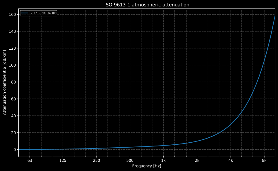```python from phonometry import environmental res = environmental.atmospheric_attenuation( [63, 125, 250, 500, 1000, 2000, 4000, 8000], temperature=20.0, relative_humidity=50.0, ) res.plot() # alpha in dB/km against frequency (needs matplotlib) ``` *On a linear decibel ordinate the coefficient stays near zero up to about 1 kHz and then climbs steeply, passing 20 dB/km near 3 kHz and reaching over 150 dB/km by 10 kHz at the reference 20 °C / 50 % RH atmosphere.*

Show the code for this figure

```python import matplotlib.pyplot as plt import numpy as np from phonometry import environmental # One line: the coefficient curve straight from the result. res = environmental.atmospheric_attenuation( np.geomspace(50.0, 10000.0, 400), temperature=20.0, relative_humidity=50.0, ) res.plot() plt.show() # Or by hand from air_attenuation (dB/m, so scale by 1000 for dB/km): freqs = np.geomspace(50.0, 10000.0, 400) fig, ax = plt.subplots() ax.semilogx(freqs, environmental.air_attenuation(freqs, 20.0, 50.0) * 1000.0) ax.set_xlabel("Frequency [Hz]") ax.set_ylabel("Attenuation coefficient alpha [dB/km]") plt.show() ```

## 2. General method of calculation (ISO 9613-2) ISO 9613-2:1996 predicts the octave-band level at a receiver **downwind** of a point source (or under the equivalent moderate temperature inversion, Clause 5). The equivalent-continuous downwind level is $$ L_{fT}(DW) = L_W + D_c - A, \qquad A = A_{div} + A_{atm} + A_{gr} + A_{bar} + A_{misc}, $$ (Eq. (3)/(4)) where $L_W$ is the octave-band sound power level, $D_c$ the directivity correction (directivity index plus a solid-angle index $D_\Omega$), and $A$ the total attenuation. The library implements the four general terms of Clause 7; the informative $A_{misc}$ (foliage, industrial sites, housing; Annex A) and reflections off vertical obstacles (Clause 7.5) are **not implemented**: the standard treats them as informative and they are left to the caller. The geometry of the screening term fixes the vocabulary: the diffraction edge splits the source-to-receiver distance into $d_{ss}$ and $d_{sr}$, and the extra path length over the edge is $z = d_{ss} + d_{sr} - d$. When the line of sight passes *above* the top edge, the standard gives $z$ a negative sign (`Barrier(line_of_sight_clear=True)`) and Eq. (14) still applies with $K_{met} = 1$: $D_z$ falls continuously from $10 \lg 3 \approx 4.8$ dB at grazing incidence to zero as the clearance deepens, never below zero. ### The four attenuation terms * **Geometrical divergence** $A_{div} = 20 \log_{10}(d/d_0) + 11$ dB, $d_0 = 1$ m (Eq. (7)): spherical spreading from a point source. Exactly 51 dB at 100 m, +6 dB per distance doubling. The $+11$ ($= 10 \lg 4\pi$) sets the level at the 1 m reference distance. * **Atmospheric absorption** $A_{atm} = \alpha\ d$ (Eq. (8)) with $\alpha$ the ISO 9613-1 coefficient, negligible at low frequency and dominant at 8 kHz over long paths. $\alpha$ is evaluated at the *exact* base-10 midband behind each nominal band label (7 943.3 Hz for "8 kHz"), the convention behind the ISO 9613-2 Table 2 coefficients (the nominal-frequency evaluation runs ~1.3 % high at 8 kHz). The ISO 9613-2 functions default to 20 °C and 70 % relative humidity (one of the Table 2 reference atmospheres the standard tabulates) while `air_attenuation` itself defaults to the ISO 9613-1 usual 50 %. * **Ground effect** $A_{gr} = A_s + A_r + A_m$ (Eq. (9)) sums a source, receiver and middle region, each from the Table 3 functions $a'/b'/c'/d'$ and its ground factor $G$ (0 = hard/reflective, 1 = porous/absorbing). A **negative** $A_{gr}$ is a net *gain* from constructive ground reflection. * **Screening** by a barrier is the diffraction insertion loss $D_z = 10 \log_{10}\big[ 3 + (C_2/\lambda)\ C_3\ z\ K_{met} \big]$ (Eq. (14)), capped at 20 dB (single edge) or 25 dB (double edge). For a top-edge barrier the ground effect of the screened path folds into it, $A_{bar} = D_z - A_{gr} \ge 0$ (Eq. (12), Note 13); for a lateral barrier $A_{bar} = D_z$ and the ground term is retained (Eq. (13)). `outdoor_propagation_attenuation` assembles the four terms into an `OutdoorAttenuation` result whose per-band arrays sum, band by band, to `a_total`, so the divergence, atmospheric, ground and barrier contributions stay separable. The stacked breakdown makes the frequency character obvious: the barrier helps most at high frequency (short wavelength) until it saturates at the cap, atmospheric absorption bites only at 8 kHz, and the ground dip lives in the mid bands.

Show the code for this figure

```python import matplotlib.pyplot as plt import numpy as np from phonometry import environmental bands = np.array([63.0, 125.0, 250.0, 500.0, 1000.0, 2000.0, 4000.0, 8000.0]) barrier = environmental.Barrier(source_to_edge=101.0, edge_to_receiver=101.0) att = environmental.outdoor_propagation_attenuation( 200.0, 1.5, 1.5, bands, ground_source=1.0, ground_middle=1.0, ground_receiver=1.0, barrier=barrier, temperature=15.0, relative_humidity=70.0, ) # One line — the same stacked breakdown with the total overlaid: att.plot() # By hand: x = np.arange(len(bands)) fig, ax = plt.subplots() # Separate positive and negative baselines: a negative term (Agr is a net # gain at 63 Hz here) stacks below zero, and the signed heights sum to a_total. pos_bottom = np.zeros(len(bands)) neg_bottom = np.zeros(len(bands)) for term, label in [(att.a_div, "Adiv — divergence"), (att.a_atm, "Aatm — atmospheric"), (att.a_gr, "Agr — ground"), (att.a_bar, "Abar — barrier")]: ax.bar(x, term, bottom=np.where(term >= 0.0, pos_bottom, neg_bottom), label=label) pos_bottom += np.maximum(term, 0.0) neg_bottom += np.minimum(term, 0.0) ax.plot(x, att.a_total, "D-", color="black", label="A — total") ax.set_xticks(x) ax.set_xticklabels([f"{b:g}" for b in bands]) ax.set_xlabel("Octave-band centre frequency [Hz]") ax.set_ylabel("Attenuation A [dB]") ax.legend() plt.show() ```

```python import numpy as np from phonometry import environmental bands = [63, 125, 250, 500, 1000, 2000, 4000, 8000] # octave-band centres [Hz] # A point source and receiver 1.5 m high, 200 m apart over porous ground # (G = 1), screened midway by a barrier that raises the path over its top edge # (dss = dsr ~ 101 m). Geometry feeds the pathlength-difference equations. barrier = environmental.Barrier(source_to_edge=101.0, edge_to_receiver=101.0) att = environmental.outdoor_propagation_attenuation( 200.0, source_height=1.5, receiver_height=1.5, frequencies=bands, ground_source=1.0, ground_middle=1.0, ground_receiver=1.0, barrier=barrier, temperature=15.0, relative_humidity=70.0, ) print(np.round(att.a_div, 1)) # [57. 57. 57. 57. 57. 57. 57. 57.] divergence print(np.round(att.a_gr, 2)) # [-4.65 2.34 13.79 9.76 1.3 -0. -0. -0. ] print(np.round(att.a_bar, 2)) # [13.78 8.89 0. 6.69 18.01 20. 20. 20. ] print(np.round(att.a_total, 1)) # [66.2 68.3 71. 73.9 77.1 78.8 82.3 96. ] att.plot() # the stacked breakdown above (needs matplotlib) # Predicted receiver level from an octave-band sound power Lw = 95 dB lw = np.full(len(bands), 95.0) lp = environmental.predicted_receiver_level( lw, 200.0, 1.5, 1.5, bands, 1.0, 1.0, 1.0, barrier=barrier, temperature=15.0, relative_humidity=70.0, ) print(np.round(lp, 1)) # [28.8 26.7 24. 21.1 17.9 16.2 12.7 -1. ] ``` `predicted_receiver_level` composes $L_{fT}(DW) = L_W + D_c - A$ with $D_c = $ `directivity_index` $+ $ `d_omega`. Pass `c0=` to subtract the meteorological correction $C_{met}$ (Eq. (21)/(22)) band by band for a long-term average; note that the standard applies $C_{met}$ to the A-weighted level, so the per-band form here is a **convenience**, not a literal reading of Clause 8. ### Ground: the alternative A-weighted method When only the A-weighted receiver level matters and the sound travels over porous or mostly-porous ground (and is not a pure tone), 7.3.2 offers a simpler closed form $A_{gr} = 4.8 - \frac{2 h_m}{d}\left(17 + \frac{300}{d}\right) \ge 0$ (Eq. (10), negative results clamped to zero), paired with the solid-angle index $D_\Omega$ (Eq. (11)) that must then be added to $D_c$. These are exposed as `ground_attenuation_alternative` and `directivity_omega`, but they are **not auto-wired** into `outdoor_propagation_attenuation` (which always uses the general per-region method of 7.3.1); combine them by hand when the alternative method is appropriate. ```python from phonometry import environmental # Alternative ground term (mean path height hm = 2 m, d = 200 m) print(round(environmental.ground_attenuation_alternative(200.0, 2.0), 2)) # 4.43 dB # Its companion solid-angle index (add to Dc when using Eq. (10)) print(round(environmental.directivity_omega(1.5, 1.5, 200.0), 2)) # 3.01 dB # Long-term meteorological correction (C0 = 2 dB) to subtract from LAT(DW) print(round(environmental.meteorological_correction(200.0, 1.5, 1.5, 2.0), 2)) # 1.7 dB ``` ### The image source behind the ground effect Every entry of Table 3 is an engineering fit to one physical picture: the receiver hears two copies of the source, the direct ray $r_1$ and a reflection that arrives exactly as if it were radiated by an **image source** mirrored below the ground plane. The two copies interfere according to the path difference $\delta = r_2 - r_1$ (about $2 h_s h_r / d$ for a grazing far-field path): in phase they add up to $+6$ dB; at $\delta = \lambda/2$ over a rigid plane they cancel into a sharp dip. Over acoustically hard ground ($G = 0$) the reflection coefficient stays close to $+1$ in every octave, the long-wavelength sum is fully constructive, and the general method duly returns $A_{gr} = -3$ dB in each band. Porous ground turns the reflection coefficient complex and angle-dependent (for a point source near grazing incidence, the spherical-wave coefficient of the Chien-Soroka solution, with a ground-wave term no plane-wave picture captures): part of the reflection flips phase, and the destructive notch lands in the 250 to 1000 Hz octaves. That notch is precisely what the $a'$ to $d'$ height-and-distance functions of Table 3 parameterize, with $G$ blending the hard and porous behaviours. The same two-ray geometry carries over to aircraft lateral attenuation and to every ray-based outdoor model; Salomons and Attenborough & Van Renterghem develop the full theory that the engineering fit compresses. A negative $A_{gr}$ (a net gain) is plain interference: the ground-reflected wave adds to the direct one. Below, a 400 Hz source 1.5 m over rigid ground builds the lobe pattern of that interference, and the level sampled on an arc converges to the two-path image-source model, dips included. [Watch the high-resolution video (WebM)](https://raw.githubusercontent.com/jmrplens/phonometry/main/.github/images/anim_fdtd_ground_effect.webm) ### `Barrier` and the screening term The `Barrier` dataclass describes the diffraction geometry directly, which is the cleanest match to Eq. (14)/(16)/(17). Single diffraction (a thin screen) leaves `edge_separation=None` ($C_3 = 1$); giving the edge spacing `e` selects double (thick-barrier) diffraction with the $C_3$ factor of Eq. (15) and the 25 dB cap. `ground_reflections_by_image=True` switches $C_2$ from 20 to 40 (reflections handled by image sources), and `lateral=True` selects vertical-edge diffraction (Eq. (13), $K_{met}=1$, ground term retained). The simulation below shows why $D_z$ grows with frequency: against the same 2.5 m screen, a 100 Hz wavefront (λ ≈ 3.4 m) diffracts over the edge and fills the shadow zone, while at 500 Hz the shadow is deep and sharp. A barrier only works when the wavelength is short next to the path difference. [Watch the high-resolution video (WebM)](https://raw.githubusercontent.com/jmrplens/phonometry/main/.github/images/anim_fdtd_barrier.webm) ### `outdoor_propagation_attenuation()` parameters | Parameter | Type / shape | Units | Range / default | Notes | | :--- | :--- | :--- | :--- | :--- | | `distance` | float | m | > 0 | Straight-line source–receiver distance $d$ | | `source_height` / `receiver_height` | float | m | ≥ 0 | $h_s$, $h_r$ above ground | | `frequencies` | 1D array | Hz | default 8 octaves 63–8000 | `DEFAULT_FREQUENCIES` | | `ground_source` / `ground_middle` / `ground_receiver` | float | — | `[0, 1]`, default `0.0` | Ground factor $G$ (0 hard, 1 porous) | | `barrier` | `Barrier` or None | — | default `None` | Screening obstacle | | `temperature` / `relative_humidity` / `pressure` | float | °C / % / kPa | 20 / 70 / 101.325 | Passed to $A_{atm}$ | | `projected_distance` | float or None | m | default $\sqrt{d^2-(h_s-h_r)^2}$ | Ground-plane $d_p$ | Returns an `OutdoorAttenuation` with `a_div`, `a_atm`, `a_gr`, `a_bar`, `a_total` and `d_omega`, all one value per band; its `.plot()` draws the stacked per-band breakdown with the total overlaid (the figure above). ### `Barrier` fields | Field | Type | Units | Default | Notes | | :--- | :--- | :--- | :--- | :--- | | `source_to_edge` | float | m | — | $d_{ss}$, source to first edge | | `edge_to_receiver` | float | m | — | $d_{sr}$, (last) edge to receiver | | `parallel_distance` | float | m | `0.0` | Component $a$ parallel to the edge | | `edge_separation` | float or None | m | `None` | $e$; given ⇒ double diffraction (25 dB cap) | | `ground_reflections_by_image` | bool | — | `False` | `True` ⇒ $C_2 = 40$ | | `lateral` | bool | — | `False` | `True` ⇒ vertical-edge diffraction (Eq. (13)) | | `line_of_sight_clear` | bool | — | `False` | `True` ⇒ the sight line passes above the top edge: the path difference takes a negative sign and Kmet = 1 (text after Eq. (16)) | ## 3. Scope, assumptions and pitfalls ### What "favourable propagation conditions" means ISO 9613-2 does not predict the level under the weather of the moment. Every equation assumes conditions **favourable to propagation** (Clause 5): wind blowing from source to receiver (within about 45° of the connecting line, at roughly 1 to 5 m/s measured 3 to 11 m above ground), or the moderate ground-based temperature inversion of a clear, calm night, which curves sound rays downward the same way. Downward refraction closes the acoustic shadow zones that upwind or neutral atmospheres would form, so the predicted $L_{fT}(DW)$ is close to the highest level the geometry can deliver: over a year the actual level is usually lower and rarely meaningfully higher. The choice is deliberate. Complaints arrive on the still nights when a distant plant is clearly audible, not on the gusty afternoons when it vanishes, and a method that predicts the audible case protects the assessment. The long-term average is recovered by subtracting $C_{met}$ (Eq. (21)/(22)), whose $C_0$ encodes how often the wind actually favours the path (about $+3$ dB when half the time is favourable, values above 2 dB already exceptional, Notes 20/22). The stated $\pm 1$ to $\pm 3$ dB accuracy (Table 5) holds under favourable conditions, for broadband sources, up to 1000 m; beyond that the standard makes no accuracy claim at all. ### Barrier pitfalls beyond the animation The screening term is the easiest one to over-trust; four fine points decide whether a real barrier delivers its computed $D_z$: * **The caps are physical, not editorial.** $D_z$ is capped at 20 dB for single and 25 dB for double diffraction no matter how tall the wall, because atmospheric turbulence scatters sound into the shadow zone and sets a ceiling that extra height cannot buy back. An insertion loss beyond roughly 20 dB is enclosure territory, not screen territory. Eq. (14) itself is a smoothed engineering curve in the tradition of Maekawa's screen chart, an empirical fit over three decades of Fresnel number $N = 2z/\lambda$. * **$K_{met}$ quietly erodes distant barriers.** The meteorological factor (Eq. (18)) discounts the screening because the same downward-curved rays that make conditions favourable also pass over the top edge. Within 100 m of source-receiver distance $K_{met} \approx 1$ (Note 17), but for a long path with a small path difference it can strip several decibels off a barrier that looks generous on the section drawing. * **Double diffraction is a modest bonus.** A thick obstacle (two edges separated by $e$) raises $C_3$ from 1 toward 3 (Eq. (15)), worth at most about $10 \lg 3 \approx 4.8$ dB extra plus the higher 25 dB cap. A building modelled as a double edge only earns that bonus if both edges really are continuous and the roof between them is closed. * **The ground effect is spent, not kept.** For a top-edge barrier the standard folds the screened path's ground effect into the diffraction: $A_{bar} = D_z - A_{gr}$ (Eq. (12), Note 13). Over porous ground that was already providing 5 to 10 dB of $A_{gr}$ in the mid bands, the *net* gain of building the barrier is correspondingly smaller than its nominal $D_z$; the two effects do not stack. An obstacle must also qualify as a barrier at all (Clause 7.4): surface density at least 10 kg/m², a closed surface without large gaps, and a horizontal extent normal to the path larger than the wavelength. A slatted fence or a short container screens far less than Eq. (14) promises. ### ISO 9613-2 or CNOSSOS-EU? Two frameworks dominate outdoor noise prediction in Europe, and they answer different questions: * **ISO 9613-2** is a general *engineering attenuation* method: given the octave-band sound power of any source you can decompose into point sources, it returns the favourable-condition receiver level. Source emission is out of scope; the sound power comes from measurement (the ISO 3740 family) or from the equipment supplier. It is the workhorse of industrial-plant and environmental impact predictions assessed with ISO 1996-2. * **CNOSSOS-EU** (Common Noise Assessment Methods in Europe) is the mandatory common framework for the strategic noise maps of the Environmental Noise Directive 2002/49/EC, adopted as its Annex II by [Commission Directive (EU) 2015/996](https://eur-lex.europa.eu/eli/dir/2015/996/oj/eng). It bundles *emission* models for road, rail and industrial sources (and delegates aircraft to ECAC Doc 29) with its own propagation part derived from the French NMPB 2008 method, producing the $L_{den}$/$L_{night}$ indicators the Directive reports. The propagation parts disagree by design, not by accident. CNOSSOS-EU evaluates every path twice, once under a homogeneous atmosphere and once under favourable (downward-refracting) conditions, and combines the two long-term with the local occurrence probability of favourable conditions per path direction; ISO 9613-2 computes only the favourable case and subtracts a scalar $C_{met}$. The ground effect in CNOSSOS-EU is built from a path-averaged ground factor over a fitted mean plane, with expressions that change between the two atmospheres, where ISO 9613-2 uses the fixed three-region Table 3. Diffraction, too, follows a different formulation that couples the ground effect on each side of the edge. Run both on the same geometry and the octave-band results can differ by several decibels, each internally consistent. The practical rule: END strategic maps and anything that must be comparable across EU member states use CNOSSOS-EU; a plant permit, a compliance prediction against a measured sound power, or work under regulations that cite ISO 9613 use this module. (ISO published a revised ISO 9613-2 in 2024; this library implements the 1996 edition, the one most national regulations and the validation literature still reference.) See the [Theory](https://jmrplens.github.io/phonometry/reference/theory/environment-transport/) page for the full derivation, the [Room Acoustics guide](https://jmrplens.github.io/phonometry/reference/api/rooms/room-acoustics/) for how $\alpha$ feeds ISO 354, and the [Occupational Noise Exposure guide](https://jmrplens.github.io/phonometry/reference/api/hearing/occupational-exposure/) for the ISO 9612 occupational exposure that consumes A-weighted levels. ## 4. Prediction reports (`.report()`) Both outdoor-propagation results render a one-page PDF **prediction** fiche. They are clearly labelled predictions, not measurements: the sheet states the meteorological and ground assumptions and, for the barrier, names the actual diffraction model behind the number. `OutdoorAttenuation.report(path)` boxes the octave-band range of the total attenuation on its own; pass a `SourceEmission` (the source sound power and directivity) to add the source power and downwind level to the table and box the A-weighted downwind level `LAT(DW)` at the receiver instead. A limit level supplied through the metadata `requirement` then adds a PASS/FAIL verdict (a lower level is better). Pass `language="es"` for the Spanish fiche. ```python import numpy as np from phonometry import ( Barrier, ReportMetadata, SourceEmission, outdoor_propagation_attenuation, ) freqs = np.array([63, 125, 250, 500, 1000, 2000, 4000, 8000], dtype=float) lw = np.array([95, 100, 103, 105, 104, 101, 95, 88], dtype=float) result = outdoor_propagation_attenuation( 200.0, 4.0, 2.0, freqs, 1.0, 1.0, 1.0, barrier=Barrier(source_to_edge=105.0, edge_to_receiver=105.0), temperature=10.0, relative_humidity=70.0, ) result.report( "outdoor_attenuation.pdf", metadata=ReportMetadata( specimen="Industrial fan plant (point source)", test_room="Nearest dwelling facade", requirement=50.0, # maximum acceptable A-weighted downwind level ), source_emission=SourceEmission(sound_power_level=lw), ) ``` Rendered examples of both fiches, regenerated with `make reports`, are kept in the repository. Click either preview to open the PDF: [](https://raw.githubusercontent.com/jmrplens/phonometry/main/.github/reports/iso9613_outdoor_attenuation_example.pdf) *Outdoor propagation fiche (`OutdoorAttenuation.report`), the A-weighted downwind level at the receiver.* Before committing the fiche, `result.plot()` draws the same per-band attenuation breakdown interactively (the stacked figure of section 2). `BarrierInsertionLoss.report(path)` boxes the mean insertion loss over the octave bands; a minimum required insertion loss supplied through `requirement` adds a PASS/FAIL verdict (a higher insertion loss is better). ```python import numpy as np from phonometry import ReportMetadata, barrier_insertion_loss freqs = np.array([63, 125, 250, 500, 1000, 2000, 4000, 8000], dtype=float) result = barrier_insertion_loss(freqs, 1.0, 50.0, 4.0, 100.0, 1.5) result.report( "barrier_insertion_loss.pdf", metadata=ReportMetadata( specimen="Roadside noise barrier, 4 m high", requirement=8.0, # minimum required mean insertion loss ), ) ``` [](https://raw.githubusercontent.com/jmrplens/phonometry/main/.github/reports/iso9613_barrier_insertion_loss_example.pdf) *Barrier insertion loss fiche (`BarrierInsertionLoss.report`), the mean insertion loss over the octave bands.* Here too `result.plot()` previews the insertion-loss spectrum of the fiche; the [ground and barriers guide](https://jmrplens.github.io/phonometry/reference/api/environment/ground-barriers/) draws the same result against the exact half-plane and coherent-ground models. ## References - Salomons, E. M. (2001). *Computational atmospheric acoustics*. Kluwer Academic Publishers. ISBN 978-1-4020-0390-5. [doi:10.1007/978-94-010-0660-6](https://doi.org/10.1007/978-94-010-0660-6). The wave-based theory (parabolic equation, fast field program, refraction and turbulence) that quantifies what the favourable-condition assumption and the $K_{met}$ factor approximate. - Attenborough, K., & Van Renterghem, T. (2021). *Predicting outdoor sound* (2nd ed.). CRC Press. [doi:10.1201/9780429470806](https://doi.org/10.1201/9780429470806). Ground impedance models, the spherical-wave reflection coefficient behind the ground dip of section 2, and the meteorological effects on barriers. - Maekawa, Z. (1968). Noise reduction by screens. *Applied Acoustics*, 1(3), 157-173. [doi:10.1016/0003-682X(68)90020-0](https://doi.org/10.1016/0003-682X(68)90020-0). The screen-attenuation chart against Fresnel number that Eq. (14)'s diffraction term descends from. - Kephalopoulos, S., Paviotti, M., & Anfosso-Lédée, F. (2012). *Common noise assessment methods in Europe (CNOSSOS-EU)* (EUR 25379 EN). Publications Office of the European Union. [doi:10.2788/31776](https://doi.org/10.2788/31776), [JRC repository](https://publications.jrc.ec.europa.eu/repository/handle/JRC72550). The common EU framework contrasted with ISO 9613-2 in section 3. - International Organization for Standardization. (1993). *Acoustics — Attenuation of sound during propagation outdoors — Part 1: Calculation of the absorption of sound by the atmosphere* (ISO 9613-1:1993). [iso.org catalogue](https://www.iso.org/standard/17426.html). The implemented pure-tone attenuation coefficient of section 1. - International Organization for Standardization. (1996). *Acoustics — Attenuation of sound during propagation outdoors — Part 2: General method of calculation* (ISO 9613-2:1996; a revised edition was published in 2024, this module implements the 1996 method). [iso.org catalogue](https://www.iso.org/standard/20649.html). The implemented attenuation chain of section 2. ## Standards ISO 9613-1:1993, *Acoustics — Attenuation of sound during propagation outdoors — Part 1: Calculation of the absorption of sound by the atmosphere*: the pure-tone attenuation coefficient $\alpha$ (Eq. (5)) with the oxygen and nitrogen relaxation frequencies (Eq. (3)/(4)), the Annex B humidity conversion and the exact Table 1 midbands (Eq. (6), Note 5). ISO 9613-2:1996, *Acoustics — Attenuation of sound during propagation outdoors — Part 2: General method of calculation*: the downwind receiver level (Eq. (3)/(4)) assembled from geometrical divergence (Eq. (7)), atmospheric absorption (Eq. (8)), the ground effect (Eq. (9), Table 3) with its A-weighted alternative (Eq. (10)/(11)), barrier screening (Eqs. (12)–(17)) and the meteorological correction (Eq. (21)/(22)). ISO 354:2003, *Acoustics — Measurement of sound absorption in a reverberation room*: only the clause 8.1.2.1 conversion $m = \alpha/(10 \lg e)$ behind `air_attenuation_m`; the reverberation-room method itself is covered in the [Room Acoustics guide](https://jmrplens.github.io/phonometry/reference/api/rooms/room-acoustics/).