Source: https://jmrplens.github.io/phonometry/perception/speech/speech-intelligibility/
# Speech Intelligibility Index (SII)
The **Speech Intelligibility Index** predicts how much of a speech signal is
audible, and therefore intelligible, to a listener in a given noise and hearing
condition. It reduces a speech spectrum, a noise spectrum and a hearing
threshold to a single number in `[0, 1]`: `0` when nothing useful reaches the
listener, `1` when the whole speech-bearing spectrum is audible. This page
covers all four band procedures of **ANSI S3.5-1997 (R2017)**: the
**one-third-octave-band method** (18 bands from 160 Hz to 8000 Hz), which is
the default and the one sections 1 to 4 work through, and the critical-band,
equally-contributing critical-band and octave-band methods of section 5.
> [!NOTE]
> **SII vs STI.** The SII predicts intelligibility from *audibility* (how much
> of the speech spectrum clears the noise and the hearing threshold at the
> listener's ear) while the STI characterises a *transmission channel*: how
> much of the speech modulation a room or sound system preserves. For the
> latter, see the [Speech Transmission Index guide](https://jmrplens.github.io/phonometry/perception/speech/speech-transmission/).
## 1. Inputs and the band-importance function
All three inputs are **equivalent spectrum levels** (ANSI S3.5-1997 clauses 3.11
and 3.55) sampled at the 18 one-third-octave band centres: the speech spectrum
level $E_i'$, the noise spectrum level $N_i'$ (both in dB SPL) and the hearing
threshold $T_i'$ (in dB HL). Each band $i$ contributes to intelligibility in
proportion to its **band-importance function** $I_i$ (ANSI S3.5-1997 Table 3,
average speech material), which sums to one across the 18 bands.
```python
from phonometry import speech
# The standard normal-effort speech spectrum (Table 3) in quiet, normal hearing.
result = speech.speech_intelligibility_index("normal")
print(round(result.sii, 3)) # 0.996 (nearly everything audible)
print(round(speech.sii.BAND_IMPORTANCE.sum(), 6)) # 1.0
result.plot() # per-band audibility and its weighted contribution (needs matplotlib)
```
With no noise and a normal hearing threshold the standard speech spectrum is
almost fully audible, so the index is close to one; the small deficit is the
listener's own **self-speech masking**.
The importance function is where the perceptual knowledge of the standard
lives. It descends from the articulation experiments behind French and
Steinberg's articulation index: listeners scored nonsense syllables heard
through filters that removed one part of the spectrum at a time, and the drop
in score measures how much intelligibility each band carries. The outcome is
strikingly unequal, and unrelated to where the speech *energy* sits: the five
bands from 1250 Hz to 3150 Hz carry about 43 % of intelligibility (the place
and manner cues of consonants live there), while the five lowest bands, 160 Hz
to 400 Hz, carry about 11 % even though they hold nearly half of the speech
power.
$I_i$ from Table 3 is the average-speech compromise; the standard's Annex B
tabulates alternative importance functions for specific test materials
(nonsense syllables, monosyllabic word lists, short passages), which shift
weight according to how much redundancy the material offers.
## 2. Masking and the band-audibility function
The procedure (ANSI S3.5-1997 clause 5) turns the inputs into a per-band
audibility. Speech masks itself downward from each band ($V_i = E_i' - 24$); the
larger of that and the external noise, $B_i$, spreads **upward** in frequency
with a level-dependent slope to give the equivalent masking spectrum level $Z_i$
(clause 5.4):
$$
Z_i = 10\log_{10}\!\left(10^{0.1 N_i'} + \sum_{kShow the code for this figure
```python
import numpy as np
import matplotlib.pyplot as plt
from phonometry import speech
speech_spectrum = speech.standard_speech_spectrum("normal")
noise = np.array([38.0, 37.0, 36.0, 34.0, 32.0, 30.0, 28.0, 26.0, 24.0,
22.0, 20.0, 18.0, 16.0, 14.0, 12.0, 10.0, 8.0, 6.0])
result = speech.speech_intelligibility_index(speech_spectrum, noise)
# One line:
result.plot()
plt.show()
# By hand, mirroring what SIIResult.plot() draws:
pos = np.arange(result.frequencies.size)
weighted = result.band_audibility * result.band_importance
fig, ax = plt.subplots()
ax.bar(pos, result.band_audibility, color="#c6dbef", label=r"Band audibility $A_i$")
ax.bar(pos, weighted / weighted.max(), width=0.5, color="#1f77b4",
label=r"Importance-weighted $I_i\,A_i$ (scaled)")
ax.set_xticks(pos)
ax.set_xticklabels([f"{f:g}" for f in result.frequencies], rotation=45, ha="right")
ax.set_xlabel("One-third-octave band [Hz]")
ax.set_ylabel("Band audibility")
ax.set_title(f"SII = {result.sii:.2f}")
ax.legend()
plt.show()
```
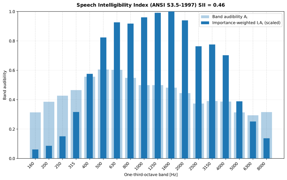
A raised hearing threshold (`threshold=`) lifts the equivalent internal noise
and lowers the index, exactly as added masking noise does. The
`SIIResult` also carries the per-band masking $Z_i$, disturbance $D_i$,
audibility $A_i$ and importance $I_i$, and its `.plot()` renders the figure
above.
The same speech and noise heard by a listener with a sloping high-frequency
loss shows what that costs, band by band:
Show the code for this figure
```python
import numpy as np
import matplotlib.pyplot as plt
from phonometry import speech
# The same speech and office noise as above, heard through a sloping
# high-frequency loss (hearing threshold levels at the 18 band centres).
speech_spectrum = speech.standard_speech_spectrum("normal")
noise = np.array([38.0, 37.0, 36.0, 34.0, 32.0, 30.0, 28.0, 26.0, 24.0,
22.0, 20.0, 18.0, 16.0, 14.0, 12.0, 10.0, 8.0, 6.0])
threshold = np.array([5.0, 5.0, 5.0, 5.0, 8.0, 10.0, 12.0, 15.0, 18.0,
22.0, 28.0, 35.0, 42.0, 48.0, 55.0, 60.0, 65.0, 70.0])
res = speech.speech_intelligibility_index(speech_spectrum, noise, threshold=threshold)
print(round(res.sii, 3)) # 0.358 (0.458 with normal hearing)
# One line: the same audibility bars, now limited by the hearing threshold.
res.plot()
plt.show()
```
The loss removes the bands that carry the consonant cues, which is why the
index falls by a fifth while the *level* of the speech has not changed at all.
This is the practical use of the SII in audiology and in noise control for
occupied spaces: a target index can be met either by lowering the noise or by
restoring audibility (amplification), and the band profile says which bands
the effort has to go into. The age-related thresholds of ISO 7029 make a
convenient population input, see [hearing threshold](https://jmrplens.github.io/phonometry/perception/hearing/hearing-threshold/).
## 4. Vocal effort
Talkers raise their voice in noise, and the standard gives four **standard
speech spectra** for the vocal efforts *normal*, *raised*, *loud* and *shout*
(ANSI S3.5-1997 Table 3). Passing the effort name selects the corresponding
spectrum; speaking louder lifts the whole spectrum and, in a fixed noise, raises
the index.
```python
import numpy as np
from phonometry import speech
# The same broadband noise, four vocal efforts.
noise = np.array([48.0, 47.0, 46.0, 44.0, 42.0, 40.0, 38.0, 36.0, 34.0,
32.0, 30.0, 28.0, 26.0, 24.0, 22.0, 20.0, 18.0, 16.0])
for effort in speech.sii.VOCAL_EFFORTS:
print(effort, round(speech.speech_intelligibility_index(effort, noise).sii, 2))
# normal 0.12 | raised 0.36 | loud 0.59 | shout 0.79
print(speech.standard_speech_spectrum("loud")[8]) # 42.16 dB SPL at 1 kHz
```
The four spectra are also available as one plottable result:
`standard_speech_spectra()` returns a `StandardSpeechSpectrum` carrying the band
centre frequencies and the per-effort band levels, and its `.plot()` draws them
as one labelled family on the one-third-octave band axis.
Show the code for this figure
```python
import numpy as np
import matplotlib.pyplot as plt
from phonometry import speech
# One line: the whole ANSI S3.5-1997 Table 3 family.
speech.standard_speech_spectra().plot()
plt.show()
# By hand, mirroring what StandardSpeechSpectrum.plot() draws:
res = speech.standard_speech_spectra()
pos = np.arange(res.frequencies.size)
fig, ax = plt.subplots()
for effort, levels in zip(res.vocal_efforts, res.levels):
ax.plot(pos, levels, "o-", label=effort.capitalize())
ax.set_xticks(pos)
ax.set_xticklabels([f"{f:g}" for f in res.frequencies], rotation=45, ha="right")
ax.set_xlabel("One-third-octave band [Hz]")
ax.set_ylabel("Speech spectrum level [dB SPL]")
ax.legend()
plt.show()
```
The same four spectra feed the index: in a fixed broadband noise, each higher
vocal effort lifts the speech spectrum and raises the SII.
Show the code for this figure
```python
import numpy as np
import matplotlib.pyplot as plt
from matplotlib.ticker import NullFormatter
from phonometry import speech
# The four ANSI S3.5-1997 Table 3 spectra and the fixed broadband noise above.
noise = np.array([48.0, 47.0, 46.0, 44.0, 42.0, 40.0, 38.0, 36.0, 34.0,
32.0, 30.0, 28.0, 26.0, 24.0, 22.0, 20.0, 18.0, 16.0])
efforts = speech.sii.VOCAL_EFFORTS # ("normal", "raised", "loud", "shout")
freqs = speech.sii.BAND_CENTERS # the 18 one-third-octave band centres
fig, (ax_s, ax_i) = plt.subplots(1, 2, figsize=(12, 5))
# Left: each higher vocal effort lifts the whole speech spectrum.
for effort in efforts:
ax_s.plot(freqs, speech.standard_speech_spectrum(effort), "o-",
label=effort.capitalize())
ax_s.set_xscale("log")
ax_s.set_xticks(list(freqs))
ax_s.set_xticklabels([f"{f:g}" for f in freqs], rotation=45, ha="right")
ax_s.xaxis.set_minor_formatter(NullFormatter())
ax_s.set_xlabel("One-third-octave band [Hz]")
ax_s.set_ylabel("Speech spectrum level [dB SPL]")
ax_s.legend()
# Right: the SII each spectrum reaches in the fixed noise.
sii = [speech.speech_intelligibility_index(e, noise).sii for e in efforts]
pos = np.arange(len(efforts))
ax_i.bar(pos, sii)
ax_i.set_xticks(pos)
ax_i.set_xticklabels([e.capitalize() for e in efforts])
ax_i.set_ylim(0.0, 1.0)
ax_i.set_ylabel("Speech Intelligibility Index")
plt.show()
```
The vocal-effort names work anywhere a speech spectrum is expected, including as
the first argument to `speech_intelligibility_index`.
## 5. The four band procedures
The standard's own title is plural, and so is the standard: ANSI S3.5-1997
defines **four** band procedures. They differ only in the band table and in how
the upward spread of masking is expressed, and `method=` selects one. The
default is the one-third-octave procedure used above. No resampling between
the four band sets is provided: each procedure expects its speech, noise and
threshold spectra sampled on its own bands.
| `method=` | Bands | Range | Constants | Spread of masking |
| :--- | ---: | :--- | :--- | :--- |
| `"critical-band"` | 21 | 100 Hz to 9500 Hz | Table 1 | between tabulated band limits |
| `"equally-contributing"` | 17 | 300 Hz to 6400 Hz | Table 2 | between tabulated band limits |
| `"one-third-octave"` | 18 | 160 Hz to 8000 Hz | Table 3 | between band centre frequencies |
| `"octave"` | 6 | 177 Hz to 11314 Hz | Table 4 | none |
Every procedure runs the same chain as section 2: self-speech masking, the
upward spread of masking, the equivalent internal noise and disturbance, the
level-distortion factor and the band-audibility function, weighted by that
procedure's own band-importance function. The masking slope is one formula
throughout, $C_i = -80 + 0.6\,(B_i + 10\log_{10} W_i)$ with $W_i$ the band
width in hertz. The critical-band and equally-contributing procedures spread
the masking from the upper limit of the masker band up to the centre frequency
of the masked band; the one-third-octave procedure writes that same geometry in
terms of the band centres, which is where its printed $0.89\,f_i/f_k$ and
$-6.353$ dB come from. The octave-band procedure carries **no** spread of
masking at all: an octave band is already wider than the spread being
modelled, so its equivalent masking spectrum level is the equivalent noise
spectrum level itself.
The four band-importance functions are one underlying distribution sampled at
four resolutions, so the wider the bands, the larger each $I_i$. Each function
sums to one, except Table 2's, which prints `0.0588` in each of its 17 bands
and so sums to 0.9996.
Show the code for this figure
```python
import numpy as np
import matplotlib.pyplot as plt
from phonometry import SII_METHODS, sii_procedure
# One line: each procedure's own .plot() steps its Ii over its band limits.
fig, ax = plt.subplots(figsize=(10, 6))
for method in SII_METHODS:
sii_procedure(method).plot(ax=ax, linewidth=1.8)
plt.show()
# By hand, mirroring what SIIProcedure.plot() draws:
fig, ax = plt.subplots()
for method in SII_METHODS:
proc = sii_procedure(method)
ii = proc.band_importance
ax.plot(proc.band_edges, np.append(ii, ii[-1]), drawstyle="steps-post",
label=method)
ax.set_xscale("log")
ax.set_xlabel("Frequency [Hz]")
ax.set_ylabel(r"Band importance $I_i$")
ax.set_ylim(bottom=0.0)
ax.legend()
plt.show()
```
Because an equivalent spectrum level is a per-hertz quantity, a white noise has
the *same* equivalent noise spectrum level in every band of every procedure,
which makes the four directly comparable:
```python
import numpy as np
from phonometry import speech
for method in speech.SII_METHODS:
n_bands = speech.sii_procedure(method).frequencies.size
result = speech.speech_intelligibility_index(
"normal", np.full(n_bands, 25.0), method=method
)
print(method, n_bands, round(result.sii, 3))
# critical-band 21 0.343
# equally-contributing 17 0.333
# one-third-octave 18 0.350
# octave 6 0.369
```
The four agree to within about 0.04 on the same listening situation. The octave
procedure reads highest because it drops the spread of masking, which is
exactly the risk it carries: feed it a strong low-frequency noise and it will
not see that noise reaching up into the speech-bearing bands.
**Which procedure to use.**
- `"one-third-octave"` is the working default: the finest resolution the
standard offers, the only table that carries all four vocal-effort speech
spectra, and the resolution measurement data usually arrives in.
- `"critical-band"` follows the auditory filter. Its 21 bands are the classical
critical bands, so it is the procedure to pair with critical-band models of
masking or loudness, and the only one that reaches down to 100 Hz.
- `"equally-contributing"` gives all 17 of its bands the same importance over
300 Hz to 6400 Hz, so the index reads directly as the fraction of
equally-important bands that are audible. That makes it fast to check by
hand, and it is the presentation closest to the articulation-index tradition
the SII grew out of.
- `"octave"` is for octave-band data, which is what sound level meters, HVAC
selections and building-acoustics reports routinely give. Use it when that is
all you have, and read it knowing the spread of masking is missing.
**An alternative band-importance function.** `band_importance=` replaces the
procedure's tabulated $I_i$ with one of your own, which is how the standard's
Annex B functions for particular speech test materials (nonsense syllables,
monosyllabic word lists, short passages) are applied. It changes the weighting
only: the audibility chain, and therefore `result.band_audibility`, is
untouched.
```python
res = speech.speech_intelligibility_index(
"normal", np.full(6, 25.0), method="octave",
band_importance=[0.0, 0.0, 1.0, 0.0, 0.0, 0.0], # all the weight at 1 kHz
)
print(round(res.sii, 3)) # 0.5 (the 1 kHz octave band alone)
```
**The tabulated constants.** `sii_procedure(method)` returns an `SIIProcedure`
carrying that procedure's band centre frequencies, band limits, band-importance
function, reference internal noise spectrum level and normal-effort standard
speech spectrum level; its `.plot()` draws the band-importance function as a
step over the band limits, which is the figure above. Tables 1, 2 and 4 print
all four vocal-effort columns in the standard, but only their normal-effort
column is carried here, so `"raised"`, `"loud"` and `"shout"` are available on
the one-third-octave procedure alone.
```python
octave = speech.sii_procedure("octave")
print(octave.frequencies) # [ 250. 500. 1000. 2000. 4000. 8000.]
print(octave.band_importance) # [0.0617 0.1671 0.2373 0.2648 0.2142 0.0549]
# Table 2 is critical bands 3 to 19 of Table 1, weighted equally.
equal = speech.sii_procedure("equally-contributing")
print(equal.band_edges[0], equal.band_edges[-1]) # 300.0 6400.0
print(equal.band_importance.sum().round(4)) # 0.9996
```
## 6. SII or STI?
The two speech metrics answer different questions from different measurements,
and each is blind to what the other captures:
| | SII (ANSI S3.5) | STI (IEC 60268-16) |
| :--- | :--- | :--- |
| Question answered | Is enough of the speech spectrum *audible* at the listener's ear? | How much of the speech *envelope* does the transmission channel preserve? |
| Inputs | Speech, noise and hearing-threshold spectra (18 one-third-octave equivalent spectrum levels) | An impulse response (indirect) or a STIPA recording through the channel (direct) |
| Band machinery | Band-importance weighting $I_i$ applied to the band audibility $A_i$ | Modulation transfer function $m(F)$ per octave band, converted to an effective SNR |
| Captures | Steady noise, upward spread of masking, hearing loss, vocal effort, level distortion | Reverberation, echoes, noise and (measured directly) non-linear processing |
| Blind to | Reverberation and any time-domain smearing: a fully audible but hopelessly reverberant channel still scores high | Individual hearing status: hearing-impaired listeners need specific corrections |
| Typical use | Audiology, hearing aids and protectors, noise-control targets at a listener position | PA systems, intercoms and rooms: rating a transmission channel end to end |
The same space can pass one and fail the other. A quiet, highly reverberant
atrium is an SII near 1 with a poor STI; a dry office flooded by ventilation
noise can rate an acceptable STI from its impulse response while the SII (and
the noise-aware STI, via `snr=` or `level=`) reveals that little of the speech
spectrum clears the noise. When both mechanisms are in play, compute both; the
inputs are cheap once the room and the noise have been measured. See the
[Speech Transmission Index guide](https://jmrplens.github.io/phonometry/perception/speech/speech-transmission/) for the STI side.
## 7. ANSI S3.5-1997 report (`.report()`)
`SIIResult.report(path)` renders a one-page PDF fiche laid out like a
speech-audibility report: a standard-basis line, an optional metadata header
block, a per-one-third-octave-band table of the equivalent speech spectrum
$E_i'$, the Table 3 band-importance function $I_i$ and the
band-audibility function $A_i$ beside the audibility and
importance-weighted contribution bars (the result's own `.plot()`), the boxed
`SII = X` single number, an optional verdict row and a footer with the fixed
disclaimer. It uses the same `ReportMetadata` container (documented under
[Insulation ratings](https://jmrplens.github.io/phonometry/buildings/insulation/insulation-ratings/#report-metadata-reportmetadata)) and
rendering engine as the ISO 717 insulation fiche; a supplied `requirement` is
read as the minimum required SII (a higher SII passes). `verbose=True` adds the
equivalent disturbance spectrum level $D_i$ column. Rendering needs
reportlab and, for the figure the fiche embeds, matplotlib (`pip install
"phonometry[report,plot]"`); only `engine="reportlab"` is supported. Pass
`language="es"` for a Spanish fiche.
```python
from phonometry import ReportMetadata, speech
res = speech.speech_intelligibility_index(speech_spectrum, noise, threshold=threshold)
res.report(
"sii_fiche.pdf",
metadata=ReportMetadata(
specimen="Conversational speech in low-frequency ambient noise",
measurement_standard="ANSI S3.5-1997",
laboratory="Phonometry Reference Laboratory",
requirement=0.75, # minimum required SII (a higher SII passes)
),
)
```
The example fiche, regenerated with `make reports`, is kept rendered in the
repository. Click the preview to open the PDF:
[](https://raw.githubusercontent.com/jmrplens/phonometry/main/.github/reports/ansi_s3_5_sii_example.pdf)
*Speech intelligibility index fiche (`SIIResult.report`), the SII with its per-band audibility.*
## Quick answers
### Which frequency bands matter most for speech intelligibility?
In the one-third-octave-band method of ANSI S3.5-1997, the band-importance function $I_i$ (Table 3, average speech material) sums to one across 18 bands from 160 Hz to 8000 Hz. The five bands from 1250 Hz to 3150 Hz carry about 43 % of intelligibility (the consonant cues), while the five lowest bands, 160 Hz to 400 Hz, carry about 11 % despite holding nearly half of the speech power.
### How is the Speech Intelligibility Index calculated?
The SII of ANSI S3.5-1997 clause 6 is the band-importance-weighted sum of the
band audibilities, $\text{SII} = \sum_i I_i A_i$, over 18 one-third-octave
bands. Each band audibility is
$A_i = \operatorname{clip}\!\left((E_i' - D_i + 15)/30,\; 0,\; 1\right)$
(clause 5.8), where $E_i'$ is the equivalent speech spectrum level and $D_i$
the equivalent disturbance combining external noise, upward spread of masking
and the equivalent internal noise. The index lies in $[0, 1]$.
### Which of the four ANSI S3.5 band procedures should I use?
ANSI S3.5-1997 defines four: critical band (21 bands, 100 Hz to 9500 Hz),
equally-contributing critical band (17 bands, 300 Hz to 6400 Hz), one-third
octave (18 bands, 160 Hz to 8000 Hz) and octave (6 bands, 250 Hz to 8000 Hz
nominal). Use `method="one-third-octave"` by default: it is the finest
resolution and the only procedure whose table carries the raised, loud and
shout speech spectra. Use `method="critical-band"` to align the index with a
critical-band (Bark) masking or loudness model, `method="equally-contributing"`
when the index should read as the fraction of equally-important bands that are
audible, and `method="octave"` when octave-band data is all that was measured,
remembering that the octave procedure carries no upward spread of masking and
so reads high under strong low-frequency noise.
### When should I use the SII instead of the STI?
Use the SII (ANSI S3.5) when the question is whether enough of the speech
spectrum is audible at the listener's ear: it captures steady noise, upward
spread of masking, hearing loss and vocal effort, but it is blind to
reverberation. The STI (IEC 60268-16) rates a transmission channel, how much
of the speech modulation a room or sound system preserves. When both
mechanisms are in play, compute both.
## See also
- [Speech Transmission Index](https://jmrplens.github.io/phonometry/perception/speech/speech-transmission/): the STI/STIPA
transmission index that the SII complements.
- [Loudness](https://jmrplens.github.io/phonometry/perception/psychoacoustics/loudness/) and
[Sound Quality Metrics](https://jmrplens.github.io/phonometry/perception/psychoacoustics/sound-quality/): loudness, sharpness and the
perception metrics of what the listener hears.
- [Filter Banks](https://jmrplens.github.io/phonometry/signals/filters/filter-banks/): the one-third-octave bands the SII is
evaluated on.
- [Levels](https://jmrplens.github.io/phonometry/signals/levels/levels/): the spectrum and band levels behind the equivalent
spectrum-level inputs.
- API reference: [`speech.sii`](https://jmrplens.github.io/phonometry/reference/api/speech/sii/).
- Theory: [Speech Intelligibility Index (ANSI S3.5)](https://jmrplens.github.io/phonometry/reference/theory/perception/#speech-intelligibility-index-ansi-s35): the band-importance weighting of ANSI S3.5 and the audibility function it multiplies.
## References
- French, N. R., & Steinberg, J. C. (1947). Factors governing the
intelligibility of speech sounds. *The Journal of the Acoustical Society of
America*, 19(1), 90-119.
[doi:10.1121/1.1916407](https://doi.org/10.1121/1.1916407).
The articulation-band experiments that the band-importance function of
section 1 descends from.
## Standards
ANSI S3.5-1997 (R2017), *American National Standard Methods for
the Calculation of the Speech Intelligibility Index*: the four band procedures
(critical band, 21 bands, Table 1; equally-contributing critical band, 17
bands, Table 2; one-third octave, 18 bands, Table 3; octave, 6 bands, Table 4)
with their band-importance functions, standard speech spectrum levels and
reference internal noise spectrum levels, and the masking, disturbance and
band-audibility procedure (clause 5) and the index (clause 6).
![The SII computation flow: three equivalent-spectrum-level inputs (speech Ei', noise Ni', hearing threshold Ti') feed the self-speech masking and spread-of-masking stage (equivalent masking spectrum level Zi), then the equivalent disturbance Di, then the band-audibility function Ai clipped to [0, 1], and finally the band-importance-weighted sum SII = sum of Ii*Ai over the 18 one-third-octave bands](https://raw.githubusercontent.com/jmrplens/phonometry/main/.github/images/diagram_speech_intelligibility_dark.svg)