Source: https://jmrplens.github.io/phonometry/guides/weighting/
# Frequency Weighting (A, B, C, D, G, AU, Z)
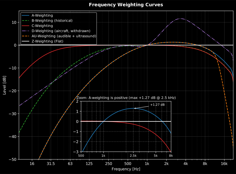
Frequency weighting curves simulate the human ear's sensitivity. A, C and Z
are specified by **IEC 61672-1:2013**; the infrasound G curve is specified by
**ISO 7196:1995**. Three more curves round out the family: the historical
**B** (ANSI S1.4-1983), the withdrawn aircraft-noise **D** (IEC 537) and
**AU** (IEC 61012) for audible sound in the presence of ultrasound
(section 4).
Show the code for this figure
```python
import matplotlib.pyplot as plt
import numpy as np
from phonometry import metrology
# Measure each curve's response: weight a centered unit impulse and take
# its spectrum (1 s buffer -> 1 Hz frequency resolution).
fs = 48000
impulse = np.zeros(fs)
impulse[fs // 2] = 1.0
freqs = np.fft.rfftfreq(fs, 1 / fs)
fig, ax = plt.subplots(figsize=(9, 5))
for curve in ("A", "B", "C", "D", "AU", "Z"):
spectrum = np.fft.rfft(metrology.weighting_filter(impulse, fs, curve=curve))
ax.semilogx(freqs[1:], 20 * np.log10(np.abs(spectrum[1:]) + np.finfo(float).eps),
label=curve)
ax.set(xlim=(10, 20000), ylim=(-80, 15),
xlabel="Frequency [Hz]", ylabel="Response [dB]")
ax.grid(True, which="both", alpha=0.3)
ax.legend()
plt.show()
```
* **A-Weighting (`A`):** Standard for environmental noise (IEC 61672-1).
* **C-Weighting (`C`):** Used for peak sound pressure and high-level noise.
* **Z-Weighting (`Z`):** Zero weighting, completely flat response.
* **G-Weighting (`G`):** Infrasound weighting per ISO 7196 (see below).
* **B-Weighting (`B`):** Historical middle curve of ANSI S1.4-1983 (section 4).
* **D-Weighting (`D`):** Aircraft-noise weighting of the withdrawn IEC 537 (section 4).
* **AU-Weighting (`AU`):** A-weighting with the IEC 61012 ultrasound cutoff (section 4).
## 1. Where the curves come from
The A and C curves are inverted equal-loudness contours, frozen into filters:
**A** approximates the inverse of the historic 40-phon contour (quiet levels,
where the ear discards bass most aggressively) and **C** the flatter ~100-phon
one (loud levels). IEC 61672-1:2013 (Annex E) defines both analytically from
four corner frequencies:
$$
f_1 = 20.599\ \text{Hz}, \quad f_2 = 107.653\ \text{Hz}, \quad
f_3 = 737.862\ \text{Hz}, \quad f_4 = 12194.217\ \text{Hz}
$$
C is a band-pass with double poles at $f_1$ and $f_4$ (2 zeros at the origin);
A adds the $f_2$ and $f_3$ poles (4 zeros), which is why it keeps falling
through the low-mids. Both are normalized to exactly 0 dB at 1 kHz. Z is the
absence of weighting. The full pole/zero derivation is in the
[Theory](https://jmrplens.github.io/phonometry/reference/theory/signal-analysis/) page.
### A short history: A, B, C and Z
The chain runs from Fletcher and Munson's 1933 equal-loudness measurements
to the first American sound level meter standard (1936), which gave meters
switchable responses so the reading could approximate loudness at different
levels: **A** from the 40-phon contour for quiet sounds, **B** from the
~70-phon contour for moderate ones, and a flat response for loud ones (the
**C** curve proper, mirroring the flatter ~100-phon contour, arrived with
the 1944 revision). Switching curves by level died in practice (readings jumped at the
switch points, and field measurements became incomparable), but A survived
alone: decades of hearing-damage and community-annoyance data had been
collected with it, and it correlates with both about as well as far more
elaborate metrics. IEC 61672-1 (first edition 2002) finished the cleanup:
B was dropped, A and C were kept with tightened tolerances, and **Z** was
introduced to replace the vaguely specified "linear" of older meters, which
varied by manufacturer. The B curve (and the aircraft-noise D curve that met
the same fate) remains available for historical data; see section 4.
### When C − A matters
Because A discards bass and C keeps it, the difference
$L_{Ceq} - L_{Aeq}$ is a one-number indicator of low-frequency content:
- **Below about 10 dB**: an ordinary broadband spectrum; the A-weighted
level rates it fairly.
- **Around 15 to 20 dB or more**: the energy is concentrated at low
frequencies (HVAC rumble, compressors, music bass through a wall). The
A-weighted level then understates the problem; look at the octave
spectrum, and below 20 Hz switch to the G curve.
- **Hearing-protector selection**: the HML method of ISO 4869-2 keys on
exactly this C-minus-A difference to decide how much low-frequency
attenuation a protector must provide (the simpler SNR method sidesteps it
by working from the C-weighted level directly).
```python
import numpy as np
from phonometry import metrology
# A 50 Hz rumble under a light broadband hiss: quiet in A, loud in C.
fs = 48000
t = np.arange(10 * fs) / fs
rng = np.random.default_rng(1)
x = 0.2 * np.sin(2 * np.pi * 50 * t) + 0.01 * rng.standard_normal(t.size)
la = metrology.leq(metrology.weighting_filter(x, fs, curve="A"))
lc = metrology.leq(metrology.weighting_filter(x, fs, curve="C"))
print(f"LAeq = {la:.1f} dB LCeq = {lc:.1f} dB C - A = {lc - la:.1f} dB")
# LAeq = 52.4 dB LCeq = 75.7 dB C - A = 23.2 dB
# C - A above 20 dB: the A-weighted number alone would hide the rumble.
```
## 2. Basic usage
```python
import numpy as np
from phonometry import metrology
# recording: a calibrated microphone capture (Pa) — recorded through your measurement chain. Synthesized here so the guide runs standalone.
fs = 48000
recording = 0.2 * np.sin(2 * np.pi * 1000 * np.arange(fs) / fs)
# Apply A-weighting to the raw recording
weighted_signal = metrology.weighting_filter(recording, fs, curve='A')
# Apply C-weighting for peak analysis
c_weighted_signal = metrology.weighting_filter(recording, fs, curve='C')
```
## 3. Infrasound: G-weighting (ISO 7196)
The **G frequency weighting** (ISO 7196:1995) rates infrasound the way A-weighting
rates audible noise. It is defined by a pole-zero configuration with 0 dB gain at
10 Hz, rises at 12 dB/octave from 1 Hz to 20 Hz (matching the steep growth of
perception in that band) and falls off at 24 dB/octave outside it. Use it for
sources with significant energy below 20 Hz (wind turbines, HVAC, blasting):
```python
import numpy as np
from phonometry import metrology
# recording: a calibrated microphone capture (Pa) — recorded through your measurement chain. Synthesized here so the guide runs standalone.
fs = 48000
recording = 0.2 * np.sin(2 * np.pi * 1000 * np.arange(fs) / fs)
g_weighted = metrology.weighting_filter(recording, fs, curve='G')
```
Show the code for this figure
```python
import matplotlib.pyplot as plt
import numpy as np
from phonometry import metrology
# Measure the G response: weight a centered unit impulse and take its
# spectrum. A long buffer gives the resolution the infrasound range
# needs (20 s -> 0.05 Hz).
fs = 4000
impulse = np.zeros(20 * fs)
impulse[impulse.size // 2] = 1.0
freqs = np.fft.rfftfreq(impulse.size, 1 / fs)
spectrum = np.fft.rfft(metrology.weighting_filter(impulse, fs, curve="G"))
fig, ax = plt.subplots(figsize=(9, 5))
ax.semilogx(freqs[1:],
20 * np.log10(np.abs(spectrum[1:]) + np.finfo(float).eps))
ax.plot(10, 0, "o", color="tab:red", label="0 dB at 10 Hz")
ax.set(xlim=(0.1, 1000), ylim=(-90, 15),
xlabel="Frequency [Hz]", ylabel="G-weighting response [dB]")
ax.grid(True, which="both", alpha=0.3)
ax.legend()
plt.show()
```
The implementation follows the ISO 7196 Table 1 pole/zero values exactly and is
verified in CI against every Table 2 nominal response value (0.25 Hz to 315 Hz).
`WeightingFilter(fs, "G")` supports the same multichannel and stateful block
processing as A/C. Levels measured with the G curve are reported as
LpG (or LGeq for the equivalent level over time).
## 4. Historical and special-purpose curves: B, D and AU
Three more curves complete the family. All three share the machinery of the
IEC 61672-1 curves (0 dB at 1 kHz, `high_accuracy` oversampling, multichannel
and stateful block processing).
### B (ANSI S1.4-1983, historical)
The middle curve of the original A/B/C level-switching scheme, drawn from
the ~70-phon equal-loudness contour. Analytically it is the C weighting with
one more zero at the origin and one extra real pole at
$f_5 = 158.49\ \text{Hz}$ (Appendix C of ANSI S1.4-1983), so it discards
less bass than A and more than C. It was dropped when IEC 61672-1 replaced
the older sound-level-meter standards; use it only to reproduce historical
data and measurements taken under older national codes (some legacy
automotive test procedures reported dB(B)). The implementation follows the
ANSI S1.4-1983 Appendix C constants and is pinned in CI against the Table IV
response values, within the strictest Table V mask (Type 0).
### D (IEC 537, withdrawn: aircraft noise)
The D weighting approximated the *perceived noisiness* contours used by the
perceived-noise-level (PNL) rating, so a plain sound level meter could
estimate aircraft noise: the +11.5 dB hump around 3.15 kHz is where jet
turbomachinery whine annoys most (it is deliberately *not* an equal-loudness
feature). NASA's aircraft-noise handbook gives the classic rule of thumb
$L_{PN} \approx L_D + 7\ \text{dB}$. IEC 537 was withdrawn and current
certification practice reports EPNL from one-third-octave analysis or plain
A-weighted levels, so `D` is provided for historical data and comparisons.
With the standard unavailable, the implementation uses the widely published
IEC 537 rational transfer function and is cross-checked against two
independent implementations (SQAT's zeros/poles and librosa's closed form,
which agree within 0.002 dB) and pinned in CI against the IEC 537 table
republished in NASA CR-3406.
```python
import numpy as np
from phonometry import metrology
# A 3.15 kHz whine sits right on the D-weighting hump: D rates it
# 10 dB *louder* than A does.
fs = 96000
t = np.arange(fs) / fs
whine = 0.1 * np.sin(2 * np.pi * 3150 * t)
ld = metrology.leq(metrology.weighting_filter(whine, fs, curve="D"))
la = metrology.leq(metrology.weighting_filter(whine, fs, curve="A"))
print(f"LD = {ld:.1f} dB LA = {la:.1f} dB")
# LD = 82.5 dB LA = 72.2 dB
```
### AU (IEC 61012, current: audible sound in the presence of ultrasound)
The only one of the three still in force. `AU` is the A weighting cascaded
with the **U** low-pass filter of IEC 61012:1990 (six poles, Table 2): flat
relative to A up to 10 kHz, then a steep cutoff (-13 dB at 16 kHz, -61.8 dB
at 40 kHz for U alone). Use it when strong ultrasonic components (ultrasonic
cleaners and welders, rodent repellers, some public-space deterrents) would
otherwise leak into an A-weighted reading through the meter's imperfect
high-frequency roll-off and overstate the *audible* exposure:
```python
import numpy as np
from phonometry import metrology
# 1 kHz tone (audible) buried under a strong 25 kHz ultrasonic component.
fs = 96000
t = np.arange(fs) / fs
audible = 0.1 * np.sin(2 * np.pi * 1000 * t)
x = audible + 1.0 * np.sin(2 * np.pi * 25000 * t)
la = metrology.leq(metrology.weighting_filter(x, fs, curve="A"))
lau = metrology.leq(metrology.weighting_filter(x, fs, curve="AU"))
la_ref = metrology.leq(metrology.weighting_filter(audible, fs, curve="A"))
print(f"LA = {la:.1f} dB LAU = {lau:.1f} dB audible alone = {la_ref:.1f} dB")
# LA = 78.6 dB LAU = 71.0 dB audible alone = 71.0 dB
# The ultrasound inflates LA by 7.6 dB; AU recovers the audible level.
```
Ultrasound only reaches a digital filter when the sample rate captures it,
so measure at 96 kHz or more (at 48 kHz there is nothing above 24 kHz to
reject); the AU design internally oversamples toward 288 kHz to keep the
steep U roll-off accurate. Levels are reported as LAU. The
implementation follows the Table 2 pole locations exactly (they reproduce
every Table 1 nominal value within 0.05 dB) and is verified in CI against
the Table 1 tolerances up to 40 kHz.
## 5. `weighting_filter()` / `WeightingFilter` parameters
| Parameter | Type | Units | Range / default | Notes |
| :--- | :--- | :--- | :--- | :--- |
| `x` | 1D or 2D array | any | non-empty | 2D is `[channels, samples]` |
| `fs` | int | Hz | > 0 | |
| `curve` | str | — | `'A'` (default), `'B'`, `'C'`, `'D'`, `'G'`, `'AU'`, `'Z'` | `'G'` per ISO 7196 (infrasound); `'B'`/`'D'` historical (§4); `'AU'` per IEC 61012 (§4); `'Z'` is a bypass |
| `high_accuracy` | bool | — | default `True` (function); class default `None` resolves to `not stateful` | Internal oversampling keeps A/C in class 1 up to 16 kHz; details in §7 |
| `stateful` | bool (class only) | — | default `False` | Carries filter state across blocks (streaming) |
| `steady_ic` | bool (class only) | — | default `False` | Steady-state initial conditions (no onset transient) |
## 6. Reusable filter object
If you weight many signals with the same parameters, design the filter once:
```python
import numpy as np
from phonometry import metrology
# recording: a calibrated microphone capture (Pa) — recorded through your measurement chain. Synthesized here so the guide runs standalone.
fs = 48000
recording = 0.2 * np.sin(2 * np.pi * 1000 * np.arange(fs) / fs)
wf = metrology.WeightingFilter(fs, "A")
signals = [recording] # your batch of recordings
for recording in signals:
weighted = wf.filter(recording)
```
## 7. High-frequency accuracy (`high_accuracy`)
A plain bilinear-transform design compresses the response near Nyquist: at
fs = 48 kHz the A-curve error at 12.5 kHz reaches −2.7 dB, outside the IEC
61672-1 **class 1** tolerance (+2.0/−2.5 dB).
By default (`high_accuracy=True`), phonometry designs and runs the weighting
filter at an internally oversampled rate (up to 8×, reaching ≥ 144 kHz at
common audio rates; a 96 kHz input runs ×2) and decimates back, keeping
the response within class 1 tolerances up to 16 kHz (error ≈ −0.5 dB at
12.5 kHz for fs = 48 kHz).
*The plain bilinear design (red) crosses the class 1 tolerance near 12.5 kHz;
the oversampled design (blue) stays close to the analytic curve.*
Show the code for this figure
```python
import matplotlib.pyplot as plt
import numpy as np
from phonometry import metrology
# Measured response of both designs at fs = 48 kHz: weight a centered
# unit impulse and take its spectrum...
fs = 48000
impulse = np.zeros(fs)
impulse[fs // 2] = 1.0
freqs = np.fft.rfftfreq(fs, 1 / fs)[1:]
# ...versus the analytic IEC 61672-1 A-curve built from the four corner
# frequencies of section 1, normalized to 0 dB at 1 kHz.
f1, f2, f3, f4 = 20.599, 107.653, 737.862, 12194.217
gain = (f4**2 * freqs**4) / ((freqs**2 + f1**2)
* np.sqrt((freqs**2 + f2**2) * (freqs**2 + f3**2))
* (freqs**2 + f4**2))
analytic = 20 * np.log10(gain / gain[np.argmin(np.abs(freqs - 1000))])
fig, ax = plt.subplots(figsize=(9, 5))
ax.semilogx(freqs, analytic, "k--", label="Analytic (IEC 61672-1)")
for high_accuracy, label in ((False, "Plain bilinear"),
(True, "Oversampled (default)")):
weighted = metrology.weighting_filter(impulse, fs, curve="A",
high_accuracy=high_accuracy)
response = 20 * np.log10(np.abs(np.fft.rfft(weighted))
+ np.finfo(float).eps)[1:]
ax.semilogx(freqs, response, label=label)
ax.set(xlim=(1000, 20000), ylim=(-12, 3),
xlabel="Frequency [Hz]", ylabel="A-weighting response [dB]")
ax.grid(True, which="both", alpha=0.3)
ax.legend()
plt.show()
```
- `high_accuracy=False` restores the legacy plain-bilinear behavior.
- For `'G'` the flag is silently ignored: its 0.25–315 Hz range is already
exact with the plain design.
- **Stateful (block) processing** always uses the legacy design: the internal
FIR resampling is incompatible with block continuity. Passing
`high_accuracy=True` together with `stateful=True` raises a `ValueError`.
```python
import numpy as np
from phonometry import metrology
# recording: a calibrated microphone capture (Pa) — recorded through your measurement chain. Synthesized here so the guide runs standalone.
fs = 48000
recording = 0.2 * np.sin(2 * np.pi * 1000 * np.arange(fs) / fs)
# Explicit legacy behavior
y = metrology.weighting_filter(recording, fs, curve="A", high_accuracy=False)
# Stateful block processing (legacy design, state carried between blocks)
wf = metrology.WeightingFilter(fs, "A", stateful=True)
blocks = [recording] # your sequence of recording blocks
for block in blocks:
weighted = wf.filter(block)
```
See [Block Processing](https://jmrplens.github.io/phonometry/guides/block-processing/) for the streaming workflow and
[Theory](https://jmrplens.github.io/phonometry/reference/theory/signal-analysis/) for the analytic curve definitions.
## 8. Verifying against the tolerance tables (IEC 61672-1, ANSI S1.4, IEC 61012)
`verify_weighting_class` checks a weighting filter against the acceptance
limits of **IEC 61672-1:2013** (Table 3). It evaluates the filter's relative
response at the *exact* base-10 frequency behind each nominal label below
Nyquist (Table 3's design goals are computed at $f = 1000 \cdot 10^{n/10}$,
e.g. 15 848.9 Hz for "16 kHz"; IEC 61672-3 tests at the same frequencies),
subtracts the design-goal weighting, and reports the performance class per
frequency with its margin in dB. A dense logarithmic sweep additionally
enforces subclause 5.5.7 *between* the nominal frequencies (the deviation
from the analytic Annex E goal must stay within the larger of the two
adjacent limits, so a resonance or notch between nominals cannot pass), and
when Table 3 rows with finite lower limits fall beyond Nyquist the verdict is
flagged `range_limited` (it then attests the checked frequencies only, not
full 10 Hz-20 kHz conformance):
```python
from phonometry import metrology
result = metrology.verify_weighting_class(metrology.WeightingFilter(48000, "A"))
print(result["overall_class"]) # 1
print(result["range_limited"]) # False
print(result["between_nominals"]) # {'worst_freq': ..., 'margin_class1_db': ...}
print(result["bands"][20])
# {'freq': 1000.0, 'class': 1, 'deviation_db': 0.0, 'margin_class1_db': 0.7, 'margin_class2_db': 1.0}
```
The Table 3 acceptance mask itself is public too: `weighting_class_limits(1)`
returns the 34 nominal frequencies with the lower/upper deviation limits (a
lower limit of `-inf` means only the upper limit applies). The limits qualify
the *deviation* from the design goal, so they are the same for A, C and Z.
The same verifier covers the section 4 curves that have published tolerance
tables. For `B` it uses ANSI S1.4-1983 (Table IV design goals, Table V
limits) and the "class" verdicts read as the standard's instrument **Types**
1 and 2. For `AU` it uses IEC 61012:1990 Table 1 (nominal A + nominal U with
the separate-unit tolerances, zero at the 1 kHz reference); IEC 61012
publishes a single tolerance set, so both margin slots agree and the verdict
is simply complies (1) or not (`None`) — note that checking the rows above
20 kHz needs `fs` ≥ 96 kHz (below that they are dropped and the verdict is
`range_limited`). `G` and `D` are rejected: ISO 7196 defines one ±1 dB
tolerance with no class structure, and the withdrawn IEC 537 left no
tolerance table behind (both curves are pinned numerically in the CI
conformance report instead).
*The oversampled A and C designs (blue, purple) stay near zero deviation,
well inside the class 1 corridor (shaded); the wider class 2 limits are
dotted. The corridor widens at the band extremes where only a one-sided
limit applies.*
Show the code for this figure
```python
import matplotlib.pyplot as plt
import numpy as np
from phonometry import metrology
freqs, lower1, upper1 = metrology.weighting_class_limits(1)
_, lower2, upper2 = metrology.weighting_class_limits(2)
lo1, lo2 = np.clip(lower1, -7, 7), np.clip(lower2, -7, 7)
fig, ax = plt.subplots(figsize=(10, 6.5))
ax.fill_between(freqs, lo1, upper1, step="mid", alpha=0.10,
label="Class 1 acceptance region")
ax.plot(freqs, upper1, drawstyle="steps-mid", label="Class 1 upper/lower limit")
ax.plot(freqs, lo1, drawstyle="steps-mid", color="C1")
ax.plot(freqs, upper2, ":", drawstyle="steps-mid", label="Class 2 upper/lower limit")
ax.plot(freqs, lo2, ":", drawstyle="steps-mid", color="C2")
for curve, marker in (("A", "o"), ("C", "s")):
bands = metrology.verify_weighting_class(metrology.WeightingFilter(48000, curve))["bands"]
f = [b["freq"] for b in bands]
dev = [b["deviation_db"] for b in bands]
ax.plot(f, dev, marker=marker, label=f"{curve} weighting deviation (48 kHz)")
ax.set(xscale="log", xlim=(10, 20000), ylim=(-7, 7),
xlabel="Frequency [Hz]", ylabel="Deviation from design goal [dB]")
ax.legend(fontsize=8, ncol=2)
plt.show()
```
## Quick answers
### When should I use C-weighting instead of A-weighting?
Use C-weighting for peak sound pressure and high-level noise, and use the difference $L_{Ceq} - L_{Aeq}$ as a low-frequency indicator: below about 10 dB the A-weighted level rates the spectrum fairly, while around 15 to 20 dB or more the energy is concentrated at low frequencies and the A-weighted level understates the problem. The HML method of ISO 4869-2 keys on exactly this C minus A difference for hearing-protector selection.
### Which weighting should I use for infrasound below 20 Hz?
Use the G frequency weighting of ISO 7196:1995, which rates infrasound the way A-weighting rates audible noise. It has 0 dB gain at 10 Hz, rises at 12 dB/octave from 1 Hz to 20 Hz and falls off at 24 dB/octave outside that band. Apply it to sources such as wind turbines, HVAC and blasting, and report levels as $L_{pG}$ (or $L_{Geq}$ for the equivalent level over time).
### Is A-weighting accurate near 16 kHz at a 48 kHz sample rate?
Not with a plain bilinear design: at fs = 48 kHz the A-curve error reaches −2.7 dB at 12.5 kHz, outside the IEC 61672-1 class 1 tolerance (+2.0/−2.5 dB). The default `high_accuracy=True` oversamples internally (up to 8×, reaching 144 kHz or more at common audio rates) and keeps the response within class 1 tolerances up to 16 kHz, with an error of about −0.5 dB at 12.5 kHz.
## References
- Fletcher, H., & Munson, W. A. (1933). Loudness, its definition, measurement
and calculation. *The Journal of the Acoustical Society of America*, 5(2),
82-108. [doi:10.1121/1.1915637](https://doi.org/10.1121/1.1915637).
The original equal-loudness measurements whose 40-phon contour the A-curve
inverts (section 1).
- International Organization for Standardization. (2023). *Acoustics —
Normal equal-loudness-level contours* (ISO 226:2023).
[iso.org catalogue](https://www.iso.org/standard/83117.html).
The modern successors of the Fletcher-Munson curves, drawn in the diagram
of section 1.
- International Electrotechnical Commission. (2013). *Electroacoustics —
Sound level meters — Part 1: Specifications* (IEC 61672-1:2013).
[IEC webstore](https://webstore.iec.ch/en/publication/5708).
The normative A/C/Z definitions, the analytic Annex E curves and the
Table 3 acceptance limits verified in section 8.
- American National Standards Institute. (1983). *Specification for Sound
Level Meters* (ANSI S1.4-1983). The historical B weighting: Appendix C
analytic definition (Formula C2), Table IV design goals and Table V
tolerance limits checked by `verify_weighting_class` in section 8.
- International Electrotechnical Commission. (1990). *Filters for the
measurement of audible sound in the presence of ultrasound*
(IEC 61012:1990). [IEC webstore](https://webstore.iec.ch/en/publication/4383).
The AU weighting: U-weighting pole locations (Table 2), nominal responses
and tolerances (Table 1) and the combined AU definition of subclause 2.2.
- International Electrotechnical Commission. (1976). *Frequency weighting
for the measurement of aircraft noise (D-weighting)* (IEC 537:1976,
withdrawn). Implemented from its published rational transfer function and
cross-checked against independent implementations (section 4).
- Bennett, R. L., & Pearsons, K. S. (1981). *Handbook of Aircraft Noise
Metrics* (NASA CR-3406). NASA.
[ntrs.nasa.gov](https://ntrs.nasa.gov/citations/19810013341).
Republishes the IEC 537 D-weighting table (Table SLD-I) used to pin the
D response in CI.
## Standards
IEC 61672-1:2013, *Electroacoustics — Sound level meters —
Part 1: Specifications*: the A, C and Z frequency-weighting curves (the
Annex E analytic definition from four corner frequencies, normalized to 0 dB
at 1 kHz), the class 1 tolerances the `high_accuracy` design keeps up to
16 kHz, and the Table 3 class 1/class 2 acceptance limits checked by
`verify_weighting_class`. ISO 7196:1995, *Acoustics — Frequency-weighting characteristic for
infrasound measurements*: the G-weighting pole/zero definition (Table 1),
verified against every Table 2 nominal response value (0.25 Hz to 315 Hz).
ANSI S1.4-1983, *Specification for Sound Level Meters*: the historical B
weighting (Appendix C, Tables IV and V). IEC 61012:1990, *Filters for the
measurement of audible sound in the presence of ultrasound*: the AU
weighting (Tables 1 and 2, subclause 2.2). IEC 537:1976 (withdrawn),
*Frequency weighting for the measurement of aircraft noise*: the D
weighting, from its published rational transfer function.