Source: https://jmrplens.github.io/phonometry/guides/surface-scattering/ # Surface Scattering, Diffusion and In-situ Absorption How a surface returns incident sound (how much it scatters away from the specular direction, how uniformly it spreads what it scatters, and how much it absorbs) is measured by a family of dedicated methods. The **reverberation room** gives the random-incidence *scattering coefficient* of a surface by comparing decays with the sample held still and rotating (ISO 17497-1). A **free-field goniometer** measures the polar response of the reflected sound and condenses it into a *diffusion coefficient* (ISO 17497-2). And out on a road, a loudspeaker and a single microphone recover the *in-situ absorption* of the pavement, either over an extended surface by subtracting the incident wave (ISO 13472-1) or through a small tube pressed onto the surface (ISO 13472-2). This page covers all four. The scattering and diffusion coefficients answer different questions and are not interchangeable: scattering is *how much* energy leaves the specular direction; diffusion is *how evenly* the reflected energy is spread over angle. ## 1. Random-incidence scattering coefficient (ISO 17497-1) The scattering coefficient $s$ is the fraction of reflected energy that does **not** leave the surface in the specular direction. ISO 17497-1 measures it in a reverberation room from four reverberation-time situations: with the test sample mounted on a turntable and held **stationary**, and with the turntable **rotating** (which averages the phase-coherent specular reflection away), each with and without a reflecting base plate. **Absorption from reverberation time (Clause 6).** Each situation converts to a Sabine absorption coefficient with the standard's own air-attenuation term: $$ \alpha = 55.3\,\frac{V}{S}\left(\frac{1}{c_2 T_2} - \frac{1}{c_1 T_1}\right) - 4\,\frac{V}{S}\,(m_2 - m_1), $$ where $V$ is the room volume, $S$ the sample area, $T$ the reverberation time, $c$ the speed of sound (Eq. (2): $c = 343.2\sqrt{(273.15+t)/293.15}$) and $m$ the power attenuation coefficient of air. The **stationary** pair gives the random-incidence absorption $\alpha_s$ (Eq. (1)); the **rotating** pair gives the specular absorption $\alpha_{spec}$ (Eq. (4)). **Scattering coefficient (Eq. (5)).** The two combine into $$ s = \frac{\alpha_{spec} - \alpha_s}{1 - \alpha_s}. $$ A fully specular surface reflects all its non-absorbed energy in the specular direction, so $\alpha_{spec} = \alpha_s$ and $s = 0$; a strong diffuser sends energy everywhere, raising $\alpha_{spec}$ towards 1 and $s$ towards 1. ```python from phonometry import materials # Four reverberation-time situations reduced to two absorption coefficients. # alpha_s from the stationary pair (Eq. 1); alpha_spec from the rotating pair # (Eq. 4). V = 200 m^3, S = 10 m^2, c = 343.2 m/s throughout. alpha_s = materials.random_incidence_absorption(200.0, 10.0, c1=343.2, T1=8.0, c2=343.2, T2=6.0) alpha_spec = materials.specular_absorption_coefficient(200.0, 10.0, c3=343.2, T3=7.5, c4=343.2, T4=5.0) s = materials.scattering_coefficient(alpha_spec, alpha_s) # Eq. 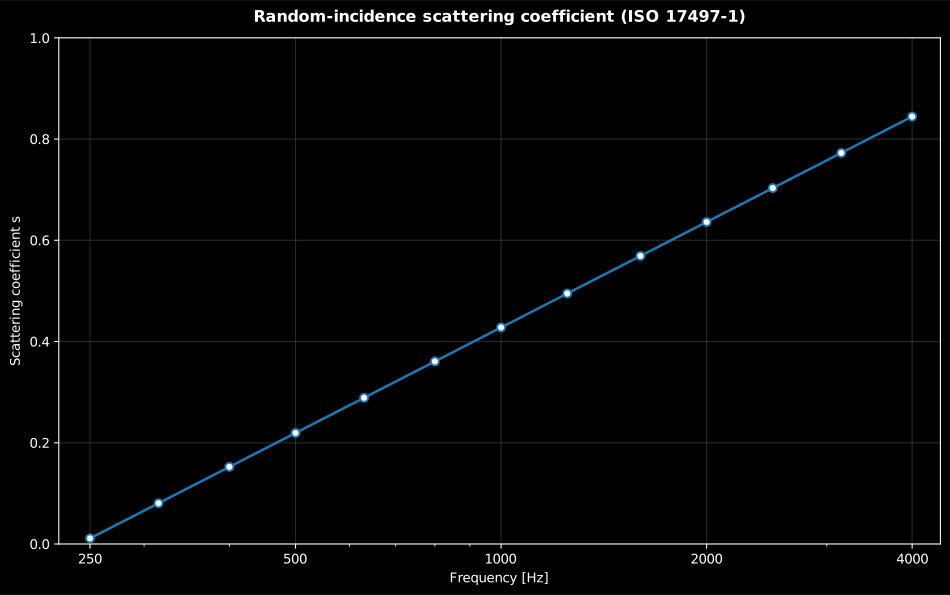(5) print(round(float(alpha_s), 4)) # 0.1343 print(round(float(alpha_spec), 4)) # 0.2148 print(round(float(s), 4)) # 0.0931 ``` Over a full one-third-octave measurement, `scattering_coefficient_spectrum` pairs the per-band $\alpha_{spec}$ and $\alpha_s$ with their band centres and returns a plottable `ScatteringResult`: ```python import numpy as np from phonometry import materials # A 13-band measurement (250-4000 Hz): the random-incidence absorption alpha_s # (stationary sample) and the specular absorption alpha_spec (rotating # turntable). A diffuser scatters more with frequency, so s(f) rises. freqs = np.array([250, 315, 400, 500, 630, 800, 1000, 1250, 1600, 2000, 2500, 3150, 4000], float) alpha_s = np.full_like(freqs, 0.10) alpha_spec = 0.11 + 0.75 * (np.log10(freqs / 250) / np.log10(4000 / 250)) result = materials.scattering_coefficient_spectrum(freqs, alpha_spec, alpha_s) print(np.round(result.scattering[[0, 6, 12]], 3)) # [0.011 0.428 0.844] result.plot() # s(f) on a log-frequency axis, 0 to 1 (needs matplotlib) ``` *The scattering coefficient climbs with frequency: at low frequency the surface relief is small compared with the wavelength and the reflection stays specular ($s \to 0$); as the wavelength shrinks the relief scatters more energy out of the specular direction ($s \to 1$).*

Show the code for this figure

```python import matplotlib.pyplot as plt import numpy as np from phonometry import materials # A 13-band measurement (250-4000 Hz): the random-incidence absorption alpha_s # (stationary sample) and the specular absorption alpha_spec (rotating # turntable). A diffuser scatters more with frequency, so s(f) rises. freqs = np.array([250, 315, 400, 500, 630, 800, 1000, 1250, 1600, 2000, 2500, 3150, 4000], float) alpha_s = np.full_like(freqs, 0.10) alpha_spec = 0.11 + 0.75 * (np.log10(freqs / 250) / np.log10(4000 / 250)) result = materials.scattering_coefficient_spectrum(freqs, alpha_spec, alpha_s) # result is the ScatteringResult computed above. One line: result.plot() plt.show() # By hand, from the result's fields, mirroring what ScatteringResult.plot() draws: fig, ax = plt.subplots() ax.semilogx(result.frequencies, result.scattering, "o-", color="#1f77b4") ax.set_xlabel("Frequency [Hz]") ax.set_ylabel("Scattering coefficient s") ax.set_ylim(0.0, 1.0) ax.set_title("Random-incidence scattering coefficient (ISO 17497-1)") plt.show() ```

**Base-plate check (Clause 6.4, Table 1).** The empty base plate must itself scatter only negligibly, or it would bias the result. ISO 17497-1 caps the base-plate scattering coefficient per one-third-octave band; the library exposes those limits and a checker. ```python from phonometry import materials # The normative per-band ceilings (Table 1): 0.05 up to 500 Hz, rising to 0.25. # materials.BASE_PLATE_BANDS is the band tuple; materials.BASE_PLATE_MAX_SCATTERING maps band -> ceiling. print(materials.BASE_PLATE_BANDS[0], materials.BASE_PLATE_MAX_SCATTERING[100]) # 100 0.05 # A base plate whose measured scattering stays under the ceiling passes silently; # an over-limit band raises a ScatteringDiffusionWarning listing the offenders. 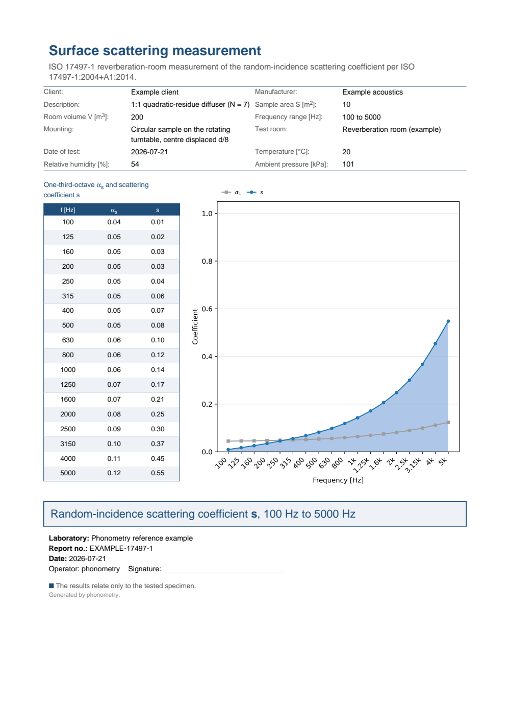materials.check_base_plate_scattering([0.02] * len(materials.BASE_PLATE_BANDS)) ``` **Test-report fiche.** `ScatteringResult.report(path)` renders a one-page accredited scattering test report (ISO 17497-1): a metadata header, the per-one-third-octave table of the random-incidence absorption $\alpha_s$ and the scattering coefficient $s$ beside the $s(f)$ curve on a categorical band axis, and a boxed characterisation headline (no pass/fail). `verbose=True` adds the specular absorption $\alpha_{spec}$ column and `language="es"` renders the Spanish fiche; it needs the report extra (`pip install phonometry[report]`). [](https://raw.githubusercontent.com/jmrplens/phonometry/main/.github/reports/iso17497_scattering_example.pdf) ## 2. Diffusion coefficient (ISO 17497-2) The diffusion coefficient $d$ measures the **spatial uniformity** of the reflected sound, not how much is scattered. A goniometer sweeps a receiver over a polar arc and records the reflected level $L_i$ at each angle; the coefficient is the normalised autocorrelation of the polar energy distribution. **Autocorrelation (Formula (5)).** For $n$ receivers at equal angular spacing, with $p_i = 10^{L_i/10}$ the band energy at receiver $i$, $$ d = \frac{\left(\sum_i p_i\right)^2 - \sum_i p_i^2} {(n-1)\,\sum_i p_i^2}. $$ A perfectly uniform polar response ($L_i$ all equal) gives $d = 1$; a single sharp specular lobe gives $d = 0$. When receivers subtend unequal solid angles, Formula (6) area-weights each energy by $N_i$ from Formula (8), and those area factors are evaluated in **radians**, which is why a 5° spacing at the zenith produces a weight near 1.57, not 51.9. The animation below runs that goniometer experiment numerically: the same plane wavefront hits a flat rigid panel and a Schroeder diffuser (an N = 7 quadratic-residue profile), and the scattered energy on the receiver arc turns a collimated specular beam (d = 0.32) into a wide fan (d = 0.63). [Watch the high-resolution video (WebM)](https://raw.githubusercontent.com/jmrplens/phonometry/main/.github/images/anim_fdtd_diffusion.webm) The single-plane response below is the far-field prediction of a published diffuser geometry: an N = 7 quadratic-residue diffuser of 6 periods, 3.6 m total width and 0.2 m maximum well depth (the "N = 7 QRD, 6 periods, 0.2 m deep" row of Cox & D'Antonio, *Acoustic Absorbers and Diffusers*, 3rd ed., Appendix B; the commercial N = 7 QRD measured by Hargreaves, Cox, Lam & D'Antonio, *J. Acoust. Soc. Am.* 108(4), 1710-1720, 2000, Table I) and its equal-footprint flat reference panel, at 1000 Hz, normal incidence, on the standard 37-point semicircle (5 deg spacing, -90 to +90 deg). The same model levels drive the phonometry conformance suite as an arithmetic oracle for Formulas (5) and (7); the external third-party anchor checks the model's band-averaged normalised diffusion against the published Appendix B BEM table in the 200-400 Hz bands (agreement within 0.01; over the full published 100-5000 Hz range the model-vs-BEM mean absolute deviation is about 0.09, because edge diffraction is outside the Fraunhofer model). The surface itself is worth drawing before predicting anything from it. `plot_qrd_geometry` turns the depth sequence into the to-scale well profile below, and a predicted `DiffuserPolarResponse` retains its geometry, so `qrd.plot_geometry()` draws the surface it was computed for. *Two of the six periods, to scale: the quadratic residues $n^2 \bmod 7$ turned into a buildable surface. The 490 Hz design frequency is what puts the deepest well at exactly 200 mm.*

Show the code for this figure

```python import matplotlib.pyplot as plt from phonometry import materials # The published N = 7 QRD: well width 3.6 m / 42, deepest well 0.2 m. depths = materials.qrd_well_depths(7, 490.0, speed_of_sound=343.0) pitch = 3.6 / 42 # 42 wells across the 3.6 m panel fin = 0.005 # thin fins, included in the pitch materials.plot_qrd_geometry(depths, pitch - fin, fin_width=fin, periods=2) plt.show() # A predicted DiffuserPolarResponse retains its geometry, so # qrd.plot_geometry() draws the profile it was computed for (all 6 periods). ```

```python from phonometry import materials # The published geometry: N = 7 QRD, 6 periods, 3.6 m wide, 0.2 m deep # (Cox & D'Antonio 3rd ed., Appendix B; Hargreaves et al. 2000, Table I). # Design frequency 490 Hz puts the deepest well at exactly 0.2 m. depths = materials.qrd_well_depths(7, 490.0) # [0, 0.05, 0.2, 0.1, ...] m qrd = materials.predict_diffuser_polar_response( 3.6 / 42, 1000.0, depths=depths, periods=6) # The flat reference panel: the same 3.6 m footprint with zero-depth wells. flat = materials.predict_diffuser_polar_response( 3.6 / 42, 1000.0, depths=[0.0] * 7, periods=6) qrd.plot() # predicted polar response, d in the title (needs matplotlib) d = materials.directional_diffusion_coefficient(qrd.levels) # Formula (5) print(round(float(d), 4)) # 0.1099 d_ref = materials.directional_diffusion_coefficient(flat.levels) print(round(float(d_ref), 4)) # 0.0049 # Normalise against the flat reference to isolate the diffuser's own effect # (Formula (7)): d_n = (d - d_ref) / (1 - d_ref). d_n = materials.normalized_diffusion_coefficient(d, d_ref) print(round(float(d_n), 4)) # 0.1055 # Random-incidence value: average the band coefficients over source positions, # with the standard's 2-D weighting (0 deg -> 1, +/-30/+/-60 deg -> 3). d_random = materials.random_incidence_diffusion( [0.5, 0.2, 0.2, 0.2, 0.2], weights=materials.TWO_DIMENSIONAL_SOURCE_WEIGHTS) print(round(float(d_random), 4)) # 0.2231 ``` `directional_diffusion` keeps the receiver angles beside the levels of a full goniometer sweep and returns a plottable `DiffusionResult`. Reusing the QRD polar levels from above: ```python import numpy as np from phonometry import materials # qrd.levels: the 37 predicted QRD levels from the example above. angles = np.arange(-90.0, 90.5, 5.0) result = materials.directional_diffusion(angles, qrd.levels) print(round(result.coefficient, 2)) # 0.11 result.plot() # polar reflected response, d in the title (needs matplotlib) ``` *The periodic QRD array splits the reflected energy into a fan of discrete grating lobes rather than one specular spike, but six repetitions of the same period concentrate the energy in those few directions, so the autocorrelation diffusion coefficient stays modest ($d \approx 0.11$). The flat reference panel collapses into the specular direction alone and drops to $d \approx 0.005$; this lobing penalty of periodic arrays is exactly why Cox & D'Antonio recommend modulated arrangements.*

Show the code for this figure

```python import matplotlib.pyplot as plt import numpy as np from phonometry import materials # qrd.levels: the 37 predicted levels L_i of the six-period N = 7 QRD from # the example above (Fraunhofer far-field model, published Cox & D'Antonio # Appendix B geometry, 1000 Hz, normal incidence) on the -90..90 deg, 5 deg # semicircle. The periodic array concentrates the energy into grating lobes, # so the Formula (5) coefficient d is modest. angles = np.arange(-90.0, 90.5, 5.0) result = materials.directional_diffusion(angles, qrd.levels) # result is the DiffusionResult computed above. One line: result.plot() plt.show() # By hand: a polar plot of the levels, with d annotated in the title. fig, ax = plt.subplots(subplot_kw={"projection": "polar"}) theta = np.radians(result.angles) ax.plot(theta, result.levels, "o-", color="#1f77b4") ax.fill(theta, result.levels, color="#1f77b4", alpha=0.15) ax.set_theta_zero_location("N") ax.set_theta_direction(-1) ax.set_thetamin(-90) ax.set_thetamax(90) ax.set_title(f"Directional diffusion d = {result.coefficient:.2f} (ISO 17497-2)") plt.show() ```

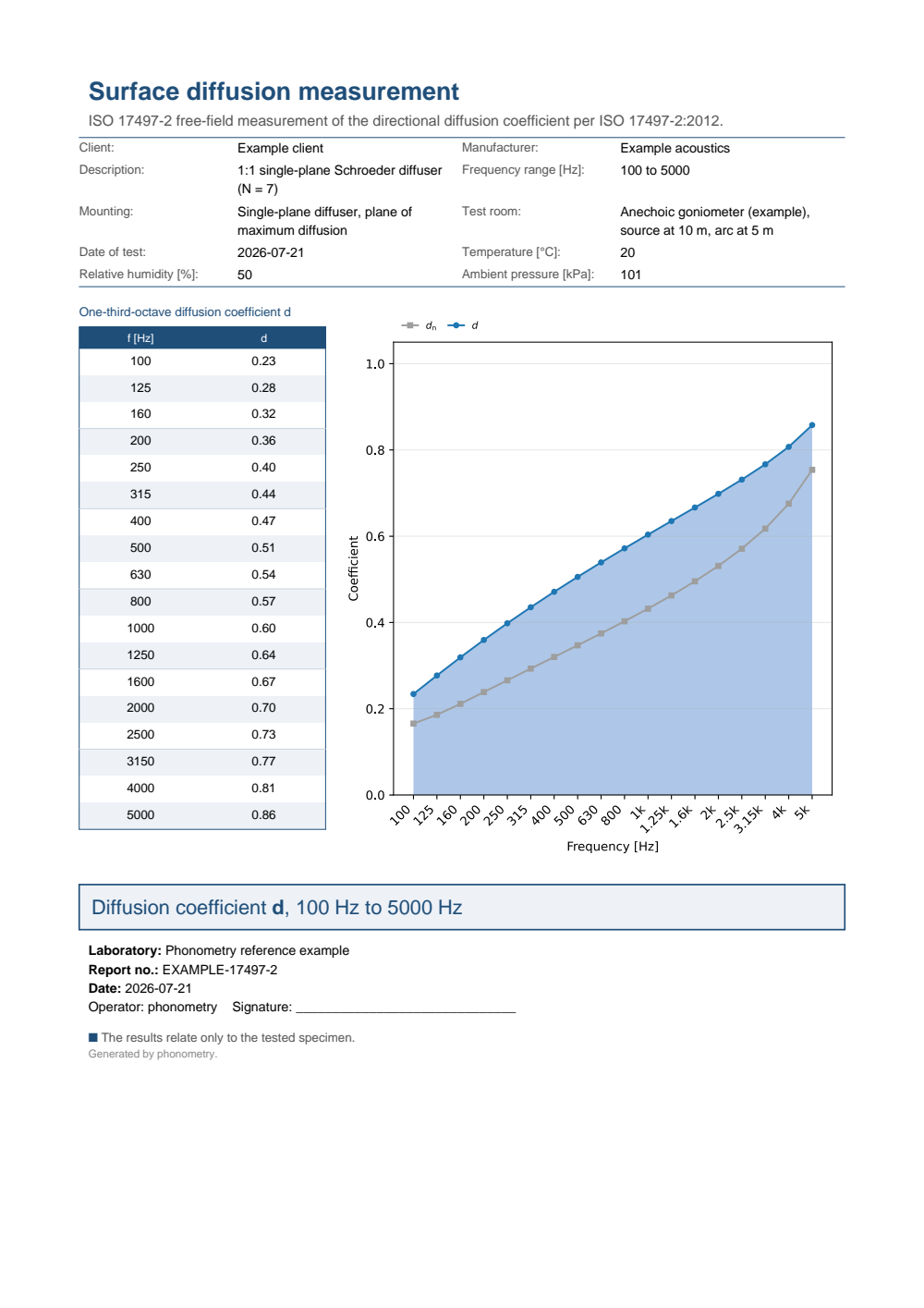
**Test-report fiche.** Collected across the one-third-octave bands, the diffusion coefficient $d(f)$ forms a `DiffusionSpectrum` (`materials.diffusion_spectrum(freqs, d, ...)`), whose `report(path)` renders a one-page diffusion test report (ISO 17497-2, Clause 8.5): the per-band table of $d$ beside the $d(f)$ band-axis curve, with a boxed characterisation headline. Per Clause 8.4 the random-incidence coefficient is itself a per-band quantity, the average of the directional coefficients over the source positions band by band (not a mean across frequency). `verbose=True` adds the normalised $d_n$ column to the table (the curve always draws $d_n$ as a companion when present). A single band's polar response is itself reportable through `DiffusionResult.report(path)`. ```python import numpy as np from phonometry import materials # One diffusion coefficient per band (here a closed-form example). In practice # each band's random-incidence d is the source-position average of the # directional coefficients: for band k, average directional_diffusion_coefficient # over the source positions with random_incidence_diffusion (Clause 8.4). freqs = np.array([250, 500, 1000, 2000, 4000], float) d = np.array([0.30, 0.45, 0.60, 0.75, 0.88]) spectrum = materials.diffusion_spectrum(freqs, d) spectrum.plot() # d(f) on the band axis (needs matplotlib) spectrum.report("diffusion.pdf") # one-page fiche (needs phonometry[report]) ``` [](https://raw.githubusercontent.com/jmrplens/phonometry/main/.github/reports/iso17497_diffusion_example.pdf) ### Predicting diffusion from a diffuser design The autocorrelation coefficient above reduces a *measured* polar response. The same coefficient can be *predicted* from the physical design of a Schroeder phase-grating diffuser, so a well-depth sequence can be graded before a sample is built. `predict_diffuser_polar_response` evaluates the single-plane Fraunhofer (far-field) model of Cox and D'Antonio: each rigid-bottom well of depth $d_n$ contributes a pressure reflection coefficient $R_n = e^{-2 j k d_n}$, and the scattered pressure at reflection angle $\theta$ for a source at incidence $\psi$ is the sum over the wells of the periodic surface (Eq. (5.8)), $$ p(\theta) = F(\theta) \sum_n R_n \, e^{\,j k x_n (\sin\psi + \sin\theta)}, $$ with $x_n$ the well centre and $k = 2\pi f / c$. The predicted polar levels $L_i = 20\lg|p(\theta_i)|$ feed the same `directional_diffusion_coefficient` as a measurement. For a quadratic residue diffuser the depth sequence follows from the prime generator $N$ and design frequency $f_0$ (Eqs. (10.2)/(10.3)): $s_n = n^2 \bmod N$ and $d_n = s_n \lambda_0 / (2N)$ with $\lambda_0 = c/f_0$. ```python import numpy as np from phonometry import materials # An N = 7 quadratic residue diffuser, design frequency 500 Hz. depths = materials.qrd_well_depths(7, 500.0) # Eqs. (10.2)/(10.3) print(np.round(depths * 100, 1)) # well depths in cm: # [ 0. 4.9 19.6 9.8 9.8 19.6 4.9] # Predicted far-field polar response at one frequency (5 repeated periods, # 10 cm wells), reduced to the ISO 17497-2 directional diffusion coefficient. surface = materials.predict_diffuser_polar_response(0.10, 2000.0, depths=depths, periods=5) print(round(surface.coefficient, 3)) # 0.210 surface.plot() # predicted polar response, d in the title (needs matplotlib) # The spectrum variant normalises band by band against the same-footprint flat # reference (Formula (7)): the flat panel maps to exactly zero, the QRD well # above it. freqs = np.array([500, 1000, 2000, 4000], float) qrd = materials.predicted_diffusion_spectrum(0.10, freqs, depths=depths, periods=5) print(np.round(qrd.normalized, 3)) # [0.352 0.275 0.208 0.073] flat = materials.predicted_diffusion_spectrum(0.10, freqs, depths=np.zeros_like(depths), periods=5) print(np.round(flat.normalized, 3)) # [0. 0. 0. 0.] ``` *Predicted from the design alone: the N = 7 QRD spreads the reflected energy far more evenly than the flat panel of the same footprint, so its predicted diffusion coefficient sits well above the near-specular flat reference across the band. This is a far-field design estimate, not a substitute for an ISO 17497-2 measurement; like every Fourier diffuser model it loses accuracy at low frequency, at grazing angles and for strongly absorbing surfaces. An arbitrary complex per-well reflection sequence can be supplied through the `reflection` argument, so an admittance or resonator-loaded surface computed elsewhere can be graded the same way.*

Show the code for this figure

```python import matplotlib.pyplot as plt import numpy as np from phonometry import materials # N = 7 QRD (design frequency 500 Hz, 10 cm wells, five periods) versus the # flat panel of the same footprint, over the one-third-octave bands. freqs = np.array([250, 315, 400, 500, 630, 800, 1000, 1250, 1600, 2000, 2500, 3150, 4000, 5000], float) depths = materials.qrd_well_depths(7, 500.0) qrd = materials.predicted_diffusion_spectrum(0.10, freqs, depths=depths, periods=5) # The DiffusionSpectrum plots the predicted d(f) directly. One line: qrd.plot() plt.show() # By hand: predicted d(f) for the QRD against the flat reference. flat = materials.predicted_diffusion_spectrum(0.10, freqs, depths=np.zeros_like(depths), periods=5, normalize=False) fig, ax = plt.subplots() ax.semilogx(freqs, qrd.diffusion, "o-", color="#1f77b4", label="N = 7 QRD design") ax.semilogx(freqs, flat.diffusion, "s--", color="#d62728", label="Flat panel") ax.set_ylim(0.0, 1.0) ax.set_xlabel("Frequency [Hz]") ax.set_ylabel("Predicted diffusion coefficient d") ax.legend() plt.show() ```

## Scattering or diffusion? Two coefficients, two jobs The two coefficients above are routinely treated as interchangeable, in product data sheets and occasionally in simulation manuals. They are not, and neither can be computed from the other. The scattering coefficient $s$ (ISO 17497-1) does **energy bookkeeping**: what fraction of the reflected energy leaves the specular direction. It says nothing about where that energy goes. The diffusion coefficient $d$ (ISO 17497-2) grades **spatial quality**: how evenly the reflected energy covers the receiver arc, one source direction at a time. It says nothing about how the energy divides between the specular lobe and the rest. A pair of counterexamples keeps them apart. A curved or tilted element that *redirects* the reflection concentrates nearly all the reflected energy into one strong lobe away from the specular direction: almost everything is non-specular, so $s$ is high, yet the beam is as collimated as a mirror's, so $d$ stays low. Conversely, a small flat panel measured at low frequency sends nearly all the reflected energy toward the specular direction, so $s$ stays near zero, yet edge diffraction spreads that reflection so broadly over the receiver arc that the measured $d$ comes out surprisingly high. High $s$ does not mean uniform; decent $d$ does not mean much energy was scattered at all. **Which one for design.** The two numbers serve different consumers: - **The scattering coefficient feeds room-acoustics simulation.** Geometrical-acoustics engines decide at every wall reflection how much energy continues specularly and how much is redistributed; the per-band random-incidence $s$ of each surface is precisely that split, which is what ISO 17497-1 was written to supply. Getting it wrong shows up as the wrong reverberation-time and clarity predictions in non-mixing rooms. - **The diffusion coefficient qualifies diffusers.** When the task is to break up an echo, a flutter or a focusing reflection, what matters is that the reflected energy is spread over angle, and $d$ measures exactly that. The normalised $d_n$ (Formula (7)) additionally subtracts the edge diffraction that every finite panel exhibits, so products of different sizes can be compared fairly. Swapping them fails in both directions: a diffusion coefficient dropped into a simulator's scattering slot biases the energy split, and a scattering coefficient quoted as proof of "diffusion" may describe a surface that merely redirects the problem reflection somewhere else. Both coefficients are one-third-octave-band functions that generally rise once the surface relief is no longer small against the wavelength; a frequency-blind single number ("scatters 90 % of the sound") is neither of them. ## 3. In-situ road absorption: subtraction technique (ISO 13472-1) Out in the field there is no reverberation room. ISO 13472-1 measures the sound absorption of a road surface (or any extended flat surface) *in situ* by firing an impulse from a loudspeaker at height $d_s$ down onto the surface and recording the impulse response at a microphone at height $d_m$. The **incident** and **reflected** components are separated in time with an Adrienne window; their transfer function gives the reflection factor and hence the absorption. **Geometrical spreading (Clause 4.1).** The reflected wave travels farther than the direct wave, so it is attenuated by the geometrical-spreading factor $$ K_r = \frac{d_s - d_m}{d_s + d_m}, $$ which equals $2/3$ for the mandatory geometry $d_s = 1.25$ m, $d_m = 0.25$ m. The absorption follows from the windowed incident and reflected spectra $H_i$, $H_r$: $$ \alpha(f) = 1 - \frac{1}{K_r^2}\left|\frac{H_r(f)}{H_i(f)}\right|^2. $$ ```python import numpy as np from phonometry import materials # A band-limited incident impulse response and a synthetic road reflection # hr = Kr * r0 * delayed(hi): a reflection of magnitude r0 = 0.4, delayed by the # extra path, and scaled by the geometrical-spreading factor Kr. fs, n = 48000.0, 4096 t = np.arange(n) / fs hi = np.zeros(n) hi[:64] = np.hanning(64) * np.cos(2.0 * np.pi * 1500.0 * t[:64]) kr = materials.geometric_spreading_factor() # (ds - dm)/(ds + dm) = 2/3 hr = kr * 0.4 * np.roll(hi, 96) # Narrow-band absorption, then reduced to one-third octaves over 250-4000 Hz. alpha = materials.insitu_absorption_coefficient(hi, hr) # 1 - (1/Kr^2)|Hr/Hi|^2 freq = np.fft.rfftfreq(n, 1.0 / fs) centres, band = materials.one_third_octave_absorption(freq, alpha) print(round(kr, 4)) # 0.6667 print(round(float(band[2]), 3)) # 0.84 (alpha = 1 - 0.4^2 = 0.84) ``` **Adrienne window (Clause 6.4).** The time window that isolates the reflection mandates only a sharp leading edge, a 5 ms flat portion and a cosine-squared or Blackman-Harris trailing edge; the exact durations are reported per measurement, not fixed, so they are configurable here. ```python from phonometry import materials # Default: 0.5 ms leading edge, 5 ms flat top, 5 ms Blackman-Harris trailing. w = materials.adrienne_window(48000.0) print(w.shape[0]) # 504 samples at 48 kHz print(round(float(w.max()), 3)) # 1.0 (flat top and edges meet at unity) ``` **End-to-end spectrum.** `insitu_absorption_spectrum` runs the whole chain (the windowed incident and reflected impulse responses to the narrow-band absorption and on to one-third-octave bands) and returns a plottable `InsituAbsorptionResult`: ```python import numpy as np from phonometry import materials from scipy.signal import firwin, lfilter # A synthetic-but-realistic measurement. hi is a unit incident impulse; the road # reflection hr = Kr * r0 * roll(hi, shift) uses the geometrical-spreading # factor Kr, a mildly frequency-dependent r0 (a gentle low-pass, so a porous # surface reflects less as frequency rises) and the reflected-path delay # shift = round(2 dm / c * fs). fs, n = 48000.0, 8192 kr = materials.geometric_spreading_factor() # (ds - dm)/(ds + dm) = 2/3 hi = np.zeros(n) hi[0] = 1.0 taps = firwin(41, 1200.0, fs=fs) taps = taps / taps.sum() shift = int(round(2.0 * 0.25 / 340.0 * fs)) # reflected-path delay 2 dm / c hr = kr * 0.85 * np.roll(lfilter(taps, 1.0, hi), shift) result = materials.insitu_absorption_spectrum(hi, hr, fs) print(result.frequencies[[0, -1]].astype(int)) # [ 250 4000] print(np.round(result.absorption[[0, 6, 12]], 2)) # [0.31 0.65 1. ] result.plot() # alpha(f) bar chart over 250-4000 Hz (needs matplotlib) ``` *The absorption rises with frequency because the surface reflects less of the high-frequency energy, exactly as the low-pass reflection factor $r_0(f)$ dictates through $\alpha = 1 - (1/K_r^2)\,|H_r/H_i|^2$.*

Show the code for this figure

```python import matplotlib.pyplot as plt import numpy as np from scipy.signal import firwin, lfilter from phonometry import materials # A synthetic-but-realistic measurement. hi is a unit incident impulse; the road # reflection hr = Kr * r0 * roll(hi, shift) uses the geometrical-spreading # factor Kr, a mildly frequency-dependent r0 (a gentle low-pass, so a porous # surface reflects less as frequency rises) and the reflected-path delay # shift = round(2 dm / c * fs). fs, n = 48000.0, 8192 kr = materials.geometric_spreading_factor() # (ds - dm)/(ds + dm) = 2/3 hi = np.zeros(n) hi[0] = 1.0 taps = firwin(41, 1200.0, fs=fs) taps = taps / taps.sum() shift = int(round(2.0 * 0.25 / 340.0 * fs)) # reflected-path delay 2 dm / c hr = kr * 0.85 * np.roll(lfilter(taps, 1.0, hi), shift) result = materials.insitu_absorption_spectrum(hi, hr, fs) # result is the InsituAbsorptionResult computed above. One line: result.plot() plt.show() # By hand: a bar chart of alpha over the one-third-octave bands. freqs = result.frequencies positions = np.arange(freqs.size) fig, ax = plt.subplots() ax.bar(positions, np.nan_to_num(result.absorption), width=0.7, color="#1f77b4") ax.set_xticks(positions) ax.set_xticklabels([f"{f:g}" for f in freqs], rotation=45, ha="right") ax.set_xlabel("Frequency [Hz]") ax.set_ylabel("Absorption coefficient alpha") ax.set_ylim(0.0, 1.0) ax.set_title("In-situ road-surface absorption (ISO 13472-1)") plt.show() ```

**Maximum sampled area (Annex A).** The finite time window limits how much of the surface contributes to the reflection. The maximum sampled area is a circle whose radius the library computes from the geometry and window width; the Annex A worked example ($d_s = 1.25$ m, $d_m = 0.25$ m, $c = 340$ m/s, 5 ms flat window) gives about 1.34 m. ```python from phonometry import materials print(round(materials.max_sampled_area_radius(5.0e-3), 3)) # 1.343 (metres) ``` ## 4. In-situ road absorption: spot method (ISO 13472-2) For smaller patches, ISO 13472-2 seals a short circular tube onto the surface and measures the absorption with the two-microphone transfer-function method of ISO 10534-2. The library provides the spot-method geometry and validity helpers; the transfer-function DSP itself is the impedance-tube routine `two_microphone_impedance` (see [Acoustic Materials](https://jmrplens.github.io/phonometry/guides/materials/)). **Plane-wave limits (Clause 5.4).** The tube supports only plane waves below $$ f_u = 0.58\,\frac{c_0}{d}, $$ with $d$ the tube diameter, and the microphone spacing $s$ must sit between $0.05\,c_0/f_{min}$ and $0.45\,c_0/f_{max}$. The reported range is the one-third-octave bands 250–1600 Hz. ```python from phonometry import materials # Upper usable frequency of a 100 mm tube and the valid spacing window. print(round(materials.spot_tube_upper_frequency(0.100, 343.0), 1)) # 1989.4 Hz s_min, s_max = materials.spot_microphone_spacing_bounds( 343.0, f_min=220.0, f_max=1800.0) print(round(s_min, 3), round(s_max, 3)) # 0.078 0.086 (metres) ``` ## References - Cox, T. J., & D'Antonio, P. (2017). *Acoustic absorbers and diffusers: Theory, design and application* (3rd ed.). CRC Press. ISBN 978-1-4987-4099-9. [doi:10.1201/9781315369211](https://doi.org/10.1201/9781315369211). The reference monograph on diffuser theory and design, by the authors behind the ISO 17497-2 diffusion-coefficient method: the scattering-versus-diffusion distinction, the measurement rigs and the design guidance this page condenses. Appendix B (Normalized diffusion coefficient table, pp. 481-485) is the published BEM anchor for the diffuser-prediction model on this page. - Hargreaves, T. J., Cox, T. J., Lam, Y. W., & D'Antonio, P. (2000). Surface diffusion coefficients for room acoustics: Free-field measures of single-plane diffusion. *The Journal of the Acoustical Society of America*, 108(4), 1710-1720. [doi:10.1121/1.1310192](https://doi.org/10.1121/1.1310192). The free-field diffusion-coefficient method behind ISO 17497-2; its Table I documents the commercial N = 7 QRD geometry (0.2 m maximum well depth) used in the worked example above. - International Organization for Standardization. (2004). *Acoustics — Sound-scattering properties of surfaces — Part 1: Measurement of the random-incidence scattering coefficient in a reverberation room* (ISO 17497-1:2004+A1:2014, the edition implemented here). [iso.org catalogue](https://www.iso.org/standard/31397.html). The turntable method implemented in section 1 of this page and the base-plate limits of the standard's Table 1. - International Organization for Standardization. (2012). *Acoustics — Sound-scattering properties of surfaces — Part 2: Measurement of the directional diffusion coefficient in a free field* (ISO 17497-2:2012). [iso.org catalogue](https://www.iso.org/standard/55293.html). The goniometer autocorrelation coefficient behind section 2 of this page, its area weighting and the normalised $d_n$. ## Standards ISO 17497-1:2004+A1:2014 (scattering coefficient), ISO 17497-2:2012 (diffusion coefficient), ISO 13472-1:2002 (in-situ absorption, extended surface), ISO 13472-2:2010 (in-situ absorption, spot method), and ISO 9613-1:1993, from which only the pure-tone attenuation coefficient α consumed by the ISO 17497-1 Clause 8 air-attenuation relations (Eqs. (2)/(3)); the full atmospheric-absorption model is covered in [Outdoor Sound Propagation](https://jmrplens.github.io/phonometry/reference/api/environment/outdoor-propagation/). Numerical conformance against the standards' worked examples and closed forms is tracked in [CONFORMANCE.md](https://jmrplens.github.io/phonometry/reference/conformance/).