Source: https://jmrplens.github.io/phonometry/guides/speech-intelligibility/ # Speech Intelligibility Index (SII) The **Speech Intelligibility Index** predicts how much of a speech signal is audible, and therefore intelligible, to a listener in a given noise and hearing condition. It reduces a speech spectrum, a noise spectrum and a hearing threshold to a single number in `[0, 1]`: `0` when nothing useful reaches the listener, `1` when the whole speech-bearing spectrum is audible. This page covers the **one-third-octave-band method** of **ANSI S3.5-1997 (R2017)**: 18 bands from 160 Hz to 8000 Hz. > [!NOTE] > **SII vs STI.** The SII predicts intelligibility from *audibility* (how much > of the speech spectrum clears the noise and the hearing threshold at the > listener's ear) while the STI characterises a *transmission channel*: how > much of the speech modulation a room or sound system preserves. For the > latter, see the [Speech Transmission Index guide](https://jmrplens.github.io/phonometry/guides/speech-transmission/). ## 1. Inputs and the band-importance function All three inputs are **equivalent spectrum levels** (ANSI S3.5-1997 clauses 3.11 and 3.55) sampled at the 18 one-third-octave band centres: the speech spectrum level `Ei'`, the noise spectrum level `Ni'` (both in dB SPL) and the hearing threshold `Ti'` (in dB HL). Each band `i` contributes to intelligibility in proportion to its **band-importance function** `Ii` (ANSI S3.5-1997 Table 3, average speech material), which sums to one across the 18 bands. ```python from phonometry import hearing # The standard normal-effort speech spectrum (Table 3) in quiet, normal hearing. result = hearing.speech_intelligibility_index("normal") print(round(result.sii, 3)) # 0.996 (nearly everything audible) print(round(hearing.sii.BAND_IMPORTANCE.sum(), 6)) # 1.0 result.plot() # per-band audibility and its weighted contribution (needs matplotlib) ``` With no noise and a normal hearing threshold the standard speech spectrum is almost fully audible, so the index is close to one; the small deficit is the listener's own **self-speech masking**. The importance function is where the perceptual knowledge of the standard lives. It descends from the articulation experiments behind French and Steinberg's articulation index: listeners scored nonsense syllables heard through filters that removed one part of the spectrum at a time, and the drop in score measures how much intelligibility each band carries. The outcome is strikingly unequal, and unrelated to where the speech *energy* sits: the five bands from 1250 Hz to 3150 Hz carry about 43 % of intelligibility (the place and manner cues of consonants live there), while the five lowest bands, 160 Hz to 400 Hz, carry about 11 % even though they hold nearly half of the speech power. `Ii` from Table 3 is the average-speech compromise; the standard's Annex B tabulates alternative importance functions for specific test materials (nonsense syllables, monosyllabic word lists, short passages), which shift weight according to how much redundancy the material offers. ## 2. Masking and the band-audibility function The procedure (ANSI S3.5-1997 clause 5) turns the inputs into a per-band audibility. Speech masks itself downward from each band (`Vi = Ei' - 24`); the larger of that and the external noise, `Bi`, spreads **upward** in frequency with a level-dependent slope to give the equivalent masking spectrum level `Zi` (clause 5.4): $$ Z_i = 10\log_{10}\!\left(10^{0.1 N_i'} + \sum_{k

Show the code for this figure

```python import numpy as np import matplotlib.pyplot as plt from phonometry import hearing speech = hearing.standard_speech_spectrum("normal") noise = np.array([38.0, 37.0, 36.0, 34.0, 32.0, 30.0, 28.0, 26.0, 24.0, 22.0, 20.0, 18.0, 16.0, 14.0, 12.0, 10.0, 8.0, 6.0]) result = hearing.speech_intelligibility_index(speech, noise) # One line: result.plot() plt.show() # By hand, mirroring what SIIResult.plot() draws: pos = np.arange(result.frequencies.size) weighted = result.band_audibility * result.band_importance fig, ax = plt.subplots() ax.bar(pos, result.band_audibility, color="#c6dbef", label=r"Band audibility $A_i$") ax.bar(pos, weighted / weighted.max(), width=0.5, color="#1f77b4", label=r"Importance-weighted $I_i A_i$ (scaled)") ax.set_xticks(pos) ax.set_xticklabels([f"{f:g}" for f in result.frequencies], rotation=45, ha="right") ax.set_xlabel("One-third-octave band [Hz]") ax.set_ylabel("Band audibility") ax.set_title(f"SII = {result.sii:.2f}") ax.legend() plt.show() ```

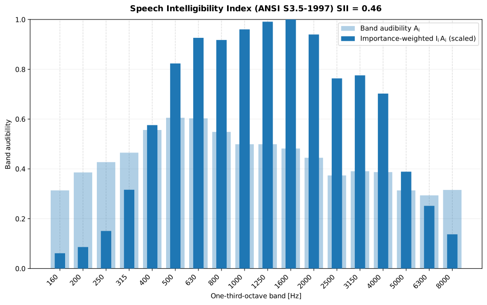
A raised hearing threshold (`threshold=`) lifts the equivalent internal noise and lowers the index, exactly as added masking noise does. The `SIIResult` also carries the per-band masking `Zi`, disturbance `Di`, audibility `Ai` and importance `Ii`, and its `.plot()` renders the figure above. The same speech and noise heard by a listener with a sloping high-frequency loss shows what that costs, band by band:

Show the code for this figure

```python import numpy as np import matplotlib.pyplot as plt from phonometry import hearing # The same speech and office noise as above, heard through a sloping # high-frequency loss (hearing threshold levels at the 18 band centres). speech = hearing.standard_speech_spectrum("normal") noise = np.array([38.0, 37.0, 36.0, 34.0, 32.0, 30.0, 28.0, 26.0, 24.0, 22.0, 20.0, 18.0, 16.0, 14.0, 12.0, 10.0, 8.0, 6.0]) threshold = np.array([5.0, 5.0, 5.0, 5.0, 8.0, 10.0, 12.0, 15.0, 18.0, 22.0, 28.0, 35.0, 42.0, 48.0, 55.0, 60.0, 65.0, 70.0]) res = hearing.speech_intelligibility_index(speech, noise, threshold=threshold) print(round(res.sii, 3)) # 0.358 (0.458 with normal hearing) # One line: the same audibility bars, now limited by the hearing threshold. res.plot() plt.show() ```

The loss removes the bands that carry the consonant cues, which is why the index falls by a fifth while the *level* of the speech has not changed at all. This is the practical use of the SII in audiology and in noise control for occupied spaces: a target index can be met either by lowering the noise or by restoring audibility (amplification), and the band profile says which bands the effort has to go into. The age-related thresholds of ISO 7029 make a convenient population input, see [hearing threshold](https://jmrplens.github.io/phonometry/guides/hearing-threshold/). ## 4. Vocal effort Talkers raise their voice in noise, and the standard gives four **standard speech spectra** for the vocal efforts *normal*, *raised*, *loud* and *shout* (ANSI S3.5-1997 Table 3). Passing the effort name selects the corresponding spectrum; speaking louder lifts the whole spectrum and, in a fixed noise, raises the index. ```python import numpy as np from phonometry import hearing # The same broadband noise, four vocal efforts. noise = np.array([48.0, 47.0, 46.0, 44.0, 42.0, 40.0, 38.0, 36.0, 34.0, 32.0, 30.0, 28.0, 26.0, 24.0, 22.0, 20.0, 18.0, 16.0]) for effort in hearing.sii.VOCAL_EFFORTS: print(effort, round(hearing.speech_intelligibility_index(effort, noise).sii, 2)) # normal 0.12 | raised 0.36 | loud 0.59 | shout 0.79 print(hearing.standard_speech_spectrum("loud")[8]) # 42.16 dB SPL at 1 kHz ``` The four spectra are also available as one plottable result: `standard_speech_spectra()` returns a `StandardSpeechSpectrum` carrying the band centre frequencies and the per-effort band levels, and its `.plot()` draws them as one labelled family on the one-third-octave band axis.

Show the code for this figure

```python import numpy as np import matplotlib.pyplot as plt from phonometry import hearing # One line: the whole ANSI S3.5-1997 Table 3 family. hearing.standard_speech_spectra().plot() plt.show() # By hand, mirroring what StandardSpeechSpectrum.plot() draws: res = hearing.standard_speech_spectra() pos = np.arange(res.frequencies.size) fig, ax = plt.subplots() for effort, levels in zip(res.vocal_efforts, res.levels): ax.plot(pos, levels, "o-", label=effort.capitalize()) ax.set_xticks(pos) ax.set_xticklabels([f"{f:g}" for f in res.frequencies], rotation=45, ha="right") ax.set_xlabel("One-third-octave band [Hz]") ax.set_ylabel("Speech spectrum level [dB SPL]") ax.legend() plt.show() ```

The same four spectra feed the index: in a fixed broadband noise, each higher vocal effort lifts the speech spectrum and raises the SII.

Show the code for this figure

```python import numpy as np import matplotlib.pyplot as plt from matplotlib.ticker import NullFormatter from phonometry import hearing # The four ANSI S3.5-1997 Table 3 spectra and the fixed broadband noise above. noise = np.array([48.0, 47.0, 46.0, 44.0, 42.0, 40.0, 38.0, 36.0, 34.0, 32.0, 30.0, 28.0, 26.0, 24.0, 22.0, 20.0, 18.0, 16.0]) efforts = hearing.sii.VOCAL_EFFORTS # ("normal", "raised", "loud", "shout") freqs = hearing.sii.BAND_CENTERS # the 18 one-third-octave band centres fig, (ax_s, ax_i) = plt.subplots(1, 2, figsize=(12, 5)) # Left: each higher vocal effort lifts the whole speech spectrum. for effort in efforts: ax_s.plot(freqs, hearing.standard_speech_spectrum(effort), "o-", label=effort.capitalize()) ax_s.set_xscale("log") ax_s.set_xticks(list(freqs)) ax_s.set_xticklabels([f"{f:g}" for f in freqs], rotation=45, ha="right") ax_s.xaxis.set_minor_formatter(NullFormatter()) ax_s.set_xlabel("One-third-octave band [Hz]") ax_s.set_ylabel("Speech spectrum level [dB SPL]") ax_s.legend() # Right: the SII each spectrum reaches in the fixed noise. sii = [hearing.speech_intelligibility_index(e, noise).sii for e in efforts] pos = np.arange(len(efforts)) ax_i.bar(pos, sii) ax_i.set_xticks(pos) ax_i.set_xticklabels([e.capitalize() for e in efforts]) ax_i.set_ylim(0.0, 1.0) ax_i.set_ylabel("Speech Intelligibility Index") plt.show() ```

The vocal-effort names work anywhere a speech spectrum is expected, including as the first argument to `speech_intelligibility_index`. ## 5. SII or STI? The two speech metrics answer different questions from different measurements, and each is blind to what the other captures: | | SII (ANSI S3.5) | STI (IEC 60268-16) | | :--- | :--- | :--- | | Question answered | Is enough of the speech spectrum *audible* at the listener's ear? | How much of the speech *envelope* does the transmission channel preserve? | | Inputs | Speech, noise and hearing-threshold spectra (18 one-third-octave equivalent spectrum levels) | An impulse response (indirect) or a STIPA recording through the channel (direct) | | Band machinery | Band-importance weighting `Ii` applied to the band audibility `Ai` | Modulation transfer function m(F) per octave band, converted to an effective SNR | | Captures | Steady noise, upward spread of masking, hearing loss, vocal effort, level distortion | Reverberation, echoes, noise and (measured directly) non-linear processing | | Blind to | Reverberation and any time-domain smearing: a fully audible but hopelessly reverberant channel still scores high | Individual hearing status: hearing-impaired listeners need specific corrections | | Typical use | Audiology, hearing aids and protectors, noise-control targets at a listener position | PA systems, intercoms and rooms: rating a transmission channel end to end | The same space can pass one and fail the other. A quiet, highly reverberant atrium is an SII near 1 with a poor STI; a dry office flooded by ventilation noise can rate an acceptable STI from its impulse response while the SII (and the noise-aware STI, via `snr=` or `level=`) reveals that little of the speech spectrum clears the noise. When both mechanisms are in play, compute both; the inputs are cheap once the room and the noise have been measured. See the [Speech Transmission Index guide](https://jmrplens.github.io/phonometry/guides/speech-transmission/) for the STI side. ## 6. ANSI S3.5-1997 report (`.report()`) `SIIResult.report(path)` renders a one-page PDF fiche laid out like a speech-audibility report: a standard-basis line, an optional metadata header block, a per-one-third-octave-band table of the equivalent speech spectrum *E*′_i, the Table 3 band-importance function *I*_i and the band-audibility function *A*_i beside the audibility and importance-weighted contribution bars (the result's own `.plot()`), the boxed `SII = X` single number, an optional verdict row and a footer with the fixed disclaimer. It uses the same `ReportMetadata` container (documented under [Field insulation](https://jmrplens.github.io/phonometry/guides/insulation-field/#report-metadata-reportmetadata)) and rendering engine as the ISO 717 insulation fiche; a supplied `requirement` is read as the minimum required SII (a higher SII passes). `verbose=True` adds the equivalent disturbance spectrum level *D*_i column. Rendering needs reportlab (`pip install phonometry[report]`); only `engine="reportlab"` is supported. Pass `language="es"` for a Spanish fiche. ```python from phonometry import hearing, ReportMetadata res = hearing.speech_intelligibility_index(speech, noise, threshold=threshold) res.report( "sii_fiche.pdf", metadata=ReportMetadata( specimen="Conversational speech in low-frequency ambient noise", measurement_standard="ANSI S3.5-1997", laboratory="Phonometry Reference Laboratory", requirement=0.75, # minimum required SII (a higher SII passes) ), ) ``` The example fiche, regenerated with `make reports`, is kept rendered in the repository. Click the preview to open the PDF: [](https://raw.githubusercontent.com/jmrplens/phonometry/main/.github/reports/ansi_s3_5_sii_example.pdf) *Speech intelligibility index fiche (`SIIResult.report`), the SII with its per-band audibility.* ## Quick answers ### Which frequency bands matter most for speech intelligibility? In the one-third-octave-band method of ANSI S3.5-1997, the band-importance function $I_i$ (Table 3, average speech material) sums to one across 18 bands from 160 Hz to 8000 Hz. The five bands from 1250 Hz to 3150 Hz carry about 43 % of intelligibility (the consonant cues), while the five lowest bands, 160 Hz to 400 Hz, carry about 11 % despite holding nearly half of the speech power. ### How is the Speech Intelligibility Index calculated? The SII of ANSI S3.5-1997 clause 6 is the band-importance-weighted sum of the band audibilities, $\text{SII} = \sum_i I_i A_i$, over 18 one-third-octave bands. Each band audibility is $A_i = \operatorname{clip}\!\left((E_i' - D_i + 15)/30,\; 0,\; 1\right)$ (clause 5.8), where $E_i'$ is the equivalent speech spectrum level and $D_i$ the equivalent disturbance combining external noise, upward spread of masking and the equivalent internal noise. The index lies in $[0, 1]$. ### When should I use the SII instead of the STI? Use the SII (ANSI S3.5) when the question is whether enough of the speech spectrum is audible at the listener's ear: it captures steady noise, upward spread of masking, hearing loss and vocal effort, but it is blind to reverberation. The STI (IEC 60268-16) rates a transmission channel, how much of the speech modulation a room or sound system preserves. When both mechanisms are in play, compute both. ## References - French, N. R., & Steinberg, J. C. (1947). Factors governing the intelligibility of speech sounds. *The Journal of the Acoustical Society of America*, 19(1), 90-119. [doi:10.1121/1.1916407](https://doi.org/10.1121/1.1916407). The articulation-band experiments that the band-importance function of section 1 descends from. ## Standards ANSI S3.5-1997 (R2017), *American National Standard Methods for the Calculation of the Speech Intelligibility Index*: the one-third-octave-band method (18 bands), band-importance function (Table 3), standard speech spectrum level and reference internal noise (Table 3), and the masking, disturbance and band-audibility procedure (clause 5) and the index (clause 6).