Source: https://jmrplens.github.io/phonometry/guides/sound-power/
# Sound Power
Sound *pressure* depends on where you stand and on the room you stand in;
sound **power** does not. The sound power level `LW` is the total acoustic
energy per second a source radiates, referenced to `P0 = 1 pW`, and it is
the device-independent **emission** descriptor that goes on a datasheet,
feeds a room prediction (EN 12354) or is checked against a noise-emission
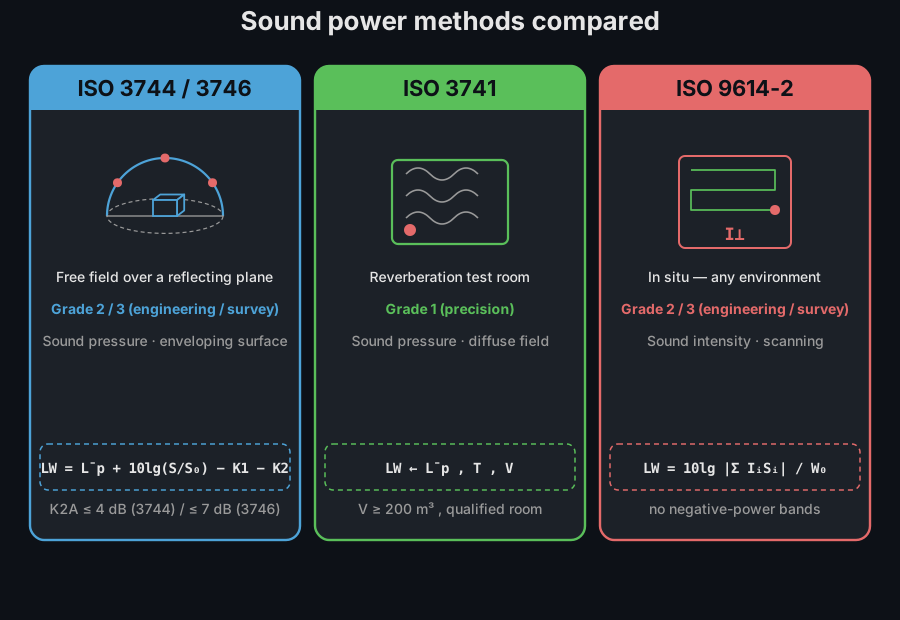
limit. This page covers the three routes phonometry implements to obtain it
and when to reach for each: an enveloping *pressure* surface in the field
(ISO 3744/3746), the diffuse field of a *reverberation room* (ISO 3741),
*intensity* scanning over a surface (ISO 9614-2), and, for the highest
accuracy, the precision grades in an *anechoic room* (ISO 3745) and by
precision *intensity* scanning (ISO 9614-3).
[Watch the high-resolution video (WebM)](https://raw.githubusercontent.com/jmrplens/phonometry/main/.github/images/anim_power_two_rooms.webm)
## Choosing a method
All deliver the same quantity, a per-band `LW` and an A-weighted total
`LWA`, but under different environments, accuracy grades and practical
constraints.
| Method | Standard | Measured quantity | Environment | Accuracy grade | Use when |
| :--- | :--- | :--- | :--- | :--- | :--- |
| Enveloping surface | **ISO 3744** (engineering) / **ISO 3746** (survey) | Sound pressure on a hemisphere or box | Essentially free field over one or more reflecting planes | Grade 2 (`σR0 ≈ 1.5 dB`) / grade 3 (`≈ 3.0 dB`) | In situ or a large room; no special test facility available |
| Reverberation room | **ISO 3741** | Sound pressure in the diffuse field | Qualified hard-walled reverberation room | Grade 1 (precision) | Highest accuracy for steady, broadband sources in a lab |
| Intensity scanning | **ISO 9614-2** | Normal sound intensity scanned over a surface | Almost any, tolerant of steady extraneous noise | Grade 2 / 3 (from per-band field indicators) | On-site with background noise, or one machine among many |
| Anechoic room | **ISO 3745** | Sound pressure on a fixed microphone array | Qualified anechoic or hemi-anechoic room | Grade 1 (precision) | Reference-grade emission in a free-field laboratory |
| Precision intensity scanning | **ISO 9614-3** | Scanned normal intensity, tighter criteria | Almost any, tolerant of steady extraneous noise | Grade 1 (precision) | Precision on-site, with the ISO 9614-3 field-indicator checks |
The pressure methods correct the surface level for the room (`K2`) and for
background noise (`K1`); the reverberation method needs a *qualified* room
but reaches precision grade; intensity rejects steady background energy at
the cost of a two-microphone probe and a per-band validity check. The rest
of the page walks each in turn.
Show the code for this figure
```python
import matplotlib.pyplot as plt
import numpy as np
from phonometry import emission
# One steady source (octave-band LW below) determined by three routes.
freqs = np.array([125.0, 250.0, 500.0, 1000.0, 2000.0, 4000.0])
lw_true = np.array([85.0, 88.0, 90.0, 89.0, 86.0, 82.0])
# ISO 3744: SPL at 10 positions on a hemisphere, r = 2 m (10 lg(S/S0) = 14 dB).
pres = emission.sound_power_pressure(np.tile(lw_true - 14.0, (10, 1)),
"hemisphere", radius=2.0,
frequencies=freqs)
# ISO 9614-2: uniform normal intensity scanned over six 0.5 m2 segments.
i_n = np.tile(10.0 ** (lw_true / 10.0) * 1e-12 / 3.0, (6, 1))
inten = emission.sound_power_intensity(i_n, np.full(6, 0.5),
frequencies=freqs, band_type="octave")
# ISO 3741: comparison against a reference source of known LW = 84 dB per band.
comp = emission.sound_power_comparison(lw_true - 20.0, np.full(6, 64.0),
np.full(6, 84.0), frequencies=freqs)
fig, ax = plt.subplots()
for res, style, ms, label in ((pres, "-o", 11, "pressure (ISO 3744)"),
(inten, "--s", 8, "intensity (ISO 9614-2)"),
(comp, ":^", 5, "reference source (ISO 3741)")):
ax.semilogx(freqs, res.sound_power_level, style, markersize=ms,
label=f"{label}: LWA = {res.sound_power_level_a:.1f} dB")
ax.set(xlabel="Frequency [Hz]", ylabel="Sound power level LW [dB]")
ax.legend()
plt.show()
```
### A decision path
The table compresses into a short sequence of questions (ISO 3740 dedicates
its Table 3 and Annex D to exactly this decision). Work through them in
order; the first match names the standard.
1. **What is the number for?** A datasheet declaration or a limit check
normally asks for engineering grade (grade 2, the preferred grade for
noise declarations); a reference source, a product ranking or a dispute
calls for precision (grade 1); a first walk-through of a noisy plant
tolerates survey grade (grade 3). Grade 1 exists only in a qualified
laboratory room (ISO 3741, ISO 3745) or via the precision intensity
methods (ISO 9614-1 at discrete points, ISO 9614-3 by scanning).
2. **Can the source travel to a laboratory?** ISO 3741 wants the source
small next to the room (volume no more than about 2 % of the room volume)
and its noise steady; ISO 3745 wants it inside a qualified anechoic or
hemi-anechoic room with a characteristic dimension below half the
measurement radius, and it is the route that also yields directivity. A
machine bolted to its foundation rules both out and leaves the in-situ
methods.
3. **How quiet and how dry is the site?** ISO 3744 needs the background at
least 6 dB below the source (preferably more than 15 dB) and
`K2 ≤ 4 dB`. If only a
3 dB margin or `K2 ≤ 7 dB` can be met, the same microphones and formulae
degrade gracefully to ISO 3746 at survey grade.
4. **Is the background the problem?** When neighbouring machines cannot be
switched off, or the margin is outright negative, the pressure methods
are out. Intensity scanning (ISO 9614-2, or ISO 9614-3 for grade 1)
tolerates steady extraneous noise even some 10 dB *above* the source,
because only the net energy flux through the surface counts; the
per-band field indicators then decide the grade actually achieved.
### What the accuracy grades mean
The grade is a claim about **reproducibility**: `σR0` is the standard
deviation you would see if different laboratories measured the same source,
each following the standard correctly. Typical A-weighted values are
`σR0 ≈ 0.5 dB` for grade 1 (ISO 3741), `1.5 dB` for grade 2 (ISO 3744,
ISO 9614-2) and `3 dB` or more for grade 3 (larger still when `K2` is
large or the spectrum is tonal). Per-band values are larger at the
spectrum edges. The `uncertainty` field of the pressure-method results
(enveloping surface and anechoic) is the expanded uncertainty
`U = 2·σtot` (95 % coverage), where
`σtot = √(σR0² + σomc²)` also folds in the operating/mounting instability
`σomc` that you estimate and pass in; the grade only bounds the method's
share of the budget.
In practice: a grade-2 `LWA` of 92.4 dB carries `U ≈ 3 dB`, so two grade-2
results 2 dB apart are statistically indistinguishable, and checking that
same source against a 93 dB limit is a coin flip. Choose the grade from the
decision the number has to support, not from the facility that happens to
be free.
## 1. Enveloping surface, sound pressure (ISO 3744 / ISO 3746)
Place the source on a reflecting plane and imagine a **measurement surface**
of area `S` wrapping it: a hemisphere for a compact source, a box (right
parallelepiped) for a large or elongated one. Sample the sound pressure
level at an array of microphone positions on that surface, energy-average
them, and the sound power follows because a diffuse-enough surface captures
all the radiated energy:
$$
\bar{L}_p = 10 \log_{10}\left( \frac{1}{N_M} \sum_i 10^{L_{pi}/10} \right), \qquad
L_W = \bar{L}_p - K_1 - K_2 + 10 \log_{10}\frac{S}{S_0},\quad S_0 = 1\ \text{m}^2 .
$$
Two corrections clean up the surface level. The **background-noise
correction** removes the energy that would have been there with the source
switched off, from the margin `ΔLp` between source-on and background levels,
$$
K_1 = -10 \log_{10}\left( 1 - 10^{-\Delta L_p/10} \right),
$$
and the **environmental correction** removes the reverberant build-up of the
test room from its equivalent absorption area `A`,
$$
K_2 = 10 \log_{10}\left( 1 + \frac{4 S}{A} \right).
$$
The surface area is a closed form of the geometry: a hemisphere is
`S = 2πr²` over one reflecting plane (halved and quartered for two and three
planes), and a one-plane box is `S = 4(ab + bc + ca)` with
`a = 0.5·l1 + d`, `b = 0.5·l2 + d`, `c = l3 + d` for measurement distance
`d`. ISO 3746 (survey) shares every formula but is coarser: fewer
microphone positions, a 3 dB background criterion instead of 6 dB, and
validity up to `K2 ≤ 7 dB` instead of 4 dB.
```python
import numpy as np
from phonometry import emission
# Octave-band SPL (dB) at the 10 hemisphere positions of ISO 3744 (Annex B),
# with the source running, plus the background spectrum with it switched off.
freqs = np.array([63, 125, 250, 500, 1000, 2000, 4000, 8000])
base = np.array([70.0, 74.0, 78.0, 80.0, 79.0, 76.0, 72.0, 66.0])
rng = np.random.default_rng(0)
levels = base + rng.normal(0.0, 0.5, size=(10, 8)) # (positions, bands)
background = np.full((10, 8), 55.0)
# ISO 3744 Annex B microphone coordinates on a radius-1.5 m hemisphere.
mic_xyz = emission.measurement_positions("hemisphere", radius=1.5, reflecting_planes=1)
print(mic_xyz.shape) # (10, 3)
res = emission.sound_power_pressure(
levels, "hemisphere", radius=1.5, reflecting_planes=1,
background_levels=background, frequencies=freqs,
reverberation_time=0.6, volume=300.0, # room data -> K2
)
print(round(res.surface_area, 2)) # 14.14 m^2 (= 2*pi*1.5^2)
print(round(float(res.environmental_correction[0]), 2)) # K2 = 2.32 dB
print(round(res.sound_power_level_a, 1)) # LWA = 92.4 dB
print(round(res.uncertainty, 1)) # U = 3.0 dB (2*sigma_R0)
print(np.round(res.sound_power_level, 1)) # per-band LW
res.plot() # sound power level bars per band, LWA in the title (needs matplotlib)
```
*One bar per band: the energy-averaged surface pressure minus the background
(`K1`) and environmental (`K2`) corrections plus the surface term
`10 lg(S/S0)` gives `LW(f)`, and the A-weighted energy sum across bands gives
the single-number `LWA` in the title.*
Show the code for this figure
```python
import matplotlib.pyplot as plt
import numpy as np
from phonometry import emission
# Octave-band SPL (dB) at the 10 hemisphere positions of ISO 3744 (Annex B),
# with the source running, plus the background spectrum with it switched off.
freqs = np.array([63, 125, 250, 500, 1000, 2000, 4000, 8000])
base = np.array([70.0, 74.0, 78.0, 80.0, 79.0, 76.0, 72.0, 66.0])
rng = np.random.default_rng(0)
levels = base + rng.normal(0.0, 0.5, size=(10, 8)) # (positions, bands)
background = np.full((10, 8), 55.0)
res = emission.sound_power_pressure(
levels, "hemisphere", radius=1.5, reflecting_planes=1,
background_levels=background, frequencies=freqs,
reverberation_time=0.6, volume=300.0, # room data -> K2
)
# res is the SoundPowerResult computed above. One line:
res.plot()
plt.show()
# By hand: a bar spectrum of LW with the A-weighted total in the title.
freqs = res.frequencies
positions = np.arange(freqs.size)
fig, ax = plt.subplots()
ax.bar(positions, res.sound_power_level, width=0.7, color="#1f77b4")
ax.set_xticks(positions)
ax.set_xticklabels([f"{f:g}" for f in freqs], rotation=45, ha="right")
ax.set_xlabel("Frequency [Hz]")
ax.set_ylabel("Sound power level LW [dB]")
ax.set_title(
f"Enveloping-surface sound power (ISO 3744) "
f"LWA = {res.sound_power_level_a:.1f} dB(A)")
plt.show()
```
The A-weighted total `LWA` is combined from the band powers with the ISO 3744
Annex E A-weighting corrections, so it needs `frequencies`. Passing the room
data (`reverberation_time` + `volume`, or `absorption_area`, or
`mean_absorption_coefficient` + `room_surface`) enables `K2`; omit it and the
field is treated as free (`K2 = 0`). If the background margin drops below the
grade criterion or `K2` exceeds the validity limit, a `SoundPowerWarning`
flags that the levels are upper bounds; the determination still returns.
### K1 and K2 pitfalls
Both corrections subtract energy from the surface level, so overestimating
either one understates the emission. That is why the standards cap them, and
why most disputes over an enveloping-surface result trace back to one of
these habits:
- **K1 has a cliff, not a slope.** At a 15 dB margin the correction is a
negligible 0.14 dB; at the 6 dB engineering criterion it is already
1.26 dB, the largest value the grade accepts. Below the criterion the
standard does not let the formula run on: `K1` is capped and the result is
reported as an upper bound. Never extrapolate the subtraction into a
smaller margin; raise the margin (quieter site, closer surface) or switch
to the intensity method.
- **K1 assumes a stationary background.** The source-off reading must be
taken at the same positions with the room in the same state, and the
background energy must be the same during both readings. A ventilation
system that cycles or a vehicle passing during either reading invalidates
the pair; the energy subtraction also assumes source and background are
incoherent, which holds for unrelated noise but not for the source's own
reflections.
- **K2 removes the average room build-up, not discrete reflections.** A
nearby wall, a trolley or another machine just outside the surface adds a
specular contribution concentrated at a few microphones. That imbalance
shows up in the apparent directivity index `DIi*`, and no room-average
correction can remove it: move the surface, remove the reflector or treat
it with absorption.
- **K2 is only as good as `A`.** With `A` from Sabine (`0.16·V/T`), errors
in the reverberation time or the volume propagate directly. At the
`K2 = 4 dB` validity limit about 60 % of the measured energy is room, not
source, and a 20 % error in `A` still moves `LW` by about 0.5 dB. Prefer a
measured `T60` over a guessed absorption coefficient, and keep the
measurement distance small enough that `K2` stays well under the limit.
### `sound_power_pressure()` parameters
| Parameter | Type | Units | Range / default | Notes |
| :--- | :--- | :--- | :--- | :--- |
| `levels_positions` | 2D array | dB | `(NM, NB)` | One row per position, one column per band (or a single A-weighted column) |
| `surface` | str | — | `'hemisphere'` / `'box'` | Measurement-surface shape |
| `radius` | float | m | > 0 (hemisphere) | Hemisphere radius `r` |
| `dimensions` | (float, float, float) | m | > 0 (box) | Reference-box `(l1, l2, l3)` |
| `distance` | float | m | > 0 (box) | Measurement distance `d` |
| `reflecting_planes` | int | — | `1` / `2` / `3`, default `1` | Halves/quarters the hemisphere area |
| `background_levels` | 2D array or spectrum | dB | `(NM, NB)`, or `(NB,)` / `(1, NB)` | Enables `K1`; a single spectrum broadcasts to every position |
| `frequencies` | 1D array | Hz | nominal band centres | Enables `LWA` (Annex E) |
| `absorption_area` | float or 1D array | m² | > 0 | `A` for `K2` (direct); per-band array → per-band `K2` |
| `reverberation_time`, `volume` | float/array, float | s, m³ | > 0 | `A = 0.16 V/T` for `K2`; per-band `T` → per-band `K2` |
| `mean_absorption_coefficient`, `room_surface` | float/array, float | —, m² | `(0,1]`, > 0 | `A = α·Sv` (Eq. A.7); per-band `α` → per-band `K2` |
| `grade` | str | — | `'engineering'` (default) / `'survey'` | ISO 3744 vs ISO 3746 |
| `omc_uncertainty` | float | dB | default `0.0` | `σomc`, operating/mounting instability, folded into `U` |
Returns a `SoundPowerResult`: `sound_power_level` (per-band `LW`),
`surface_pressure_level` (`Lp` after K1/K2), `mean_pressure_level`,
`background_correction`/`environmental_correction` (`K1`/`K2`),
`directivity_index` (apparent `DIi*` per microphone position **and** frequency
band, shape `(NM, NB)`; ISO 3744 clause 8.6), `surface_area`,
`sound_power_level_a` (`LWA`), `uncertainty` (expanded, 95 %) and `grade`.
`measurement_positions('hemisphere', radius=…, reflecting_planes=…, tones=…,
grade=…)` returns the normative `(N, 3)` microphone coordinates (Table B.1 for
tonal sources, B.2 for broadband).
## 2. Reverberation room, precision grade (ISO 3741)
In a qualified hard-walled **reverberation room** the field is diffuse, so a
handful of microphones sample the whole radiated energy and the method
reaches grade 1. The sound power comes from the mean room level `Lp(ST)`,
the Sabine absorption area `A = (55.26/c)·(V/T60)` and a chain of small
corrections (ISO 3741 Eq. 20):
$$
L_W = \bar{L}_p + 10 \log_{10}\frac{A}{A_0} + 4.34\ \frac{A}{S}
+ 10 \log_{10}\left( 1 + \frac{S c}{8 V f} \right) + C_1 + C_2 - 6 .
$$
The bracketed term is the **Waterhouse correction**: near the room
boundaries the sound energy density is higher than in the interior, and
this term (which vanishes as frequency grows) restores the energy the
interior microphones miss. `C1` (reference-quantity) and `C2`
(radiation-impedance) carry the result to the reference meteorological
conditions of 23 °C and 101.325 kPa,
$$
C_1 = -10 \log_{10}\frac{p_s}{p_{s0}} + 5 \log_{10}\frac{273.15 + \theta}{314}, \qquad
C_2 = -10 \log_{10}\frac{p_s}{p_{s0}} + 15 \log_{10}\frac{273.15 + \theta}{296},
$$
with the speed of sound `c = 20.05·√(273 + θ)`. The **comparison method**
replaces the absorption-area, Waterhouse and `C1` terms by a reference sound
source of known power `LW(RSS)` measured in the same room, so the room need
not be characterised: `LW = LW(RSS) + (Lp(ST) − Lp(RSS) + C2)`.
```python
import numpy as np
from phonometry import emission
# One-third-octave mean room SPL (dB), 100 Hz - 10 kHz, and the room's T60.
freqs = np.array([100, 125, 160, 200, 250, 315, 400, 500, 630, 800, 1000,
1250, 1600, 2000, 2500, 3150, 4000, 5000, 6300, 8000, 10000],
dtype=float)
lp = np.linspace(80.0, 70.0, freqs.size)
t60 = np.full(freqs.size, 2.0)
rev = emission.sound_power_reverberation(
lp, t60, volume=200.0, surface_area=220.0, frequencies=freqs,
temperature=20.0, static_pressure=101.0,
)
print(round(rev.speed_of_sound, 1)) # c = 343.2 m/s
print(round(float(rev.absorption_area[0]), 1)) # A = 16.1 m^2 at 100 Hz
print(round(float(rev.waterhouse_correction[0]), 2)) # 1.68 dB at 100 Hz
print(round(float(rev.sound_power_level[0]), 1)) # LW = 87.9 dB
print(round(rev.sound_power_level_a, 1)) # LWA = 92.1 dB
# Comparison method: a reference source of known LW measured at the same spots.
lw_rss = np.full(freqs.size, 85.0)
lp_rss = np.linspace(78.0, 69.0, freqs.size)
cmp = emission.sound_power_comparison(lp, lp_rss, lw_rss, frequencies=freqs, temperature=20.0)
print(round(float(cmp.sound_power_level[0]), 1), cmp.method) # 86.9 comparison
rev.plot() # reverberation-room LW spectrum, LWA in the title (needs matplotlib)
```
*The mean room level carried through the absorption-area, Waterhouse and
meteorological terms of Eq. 20 gives the one-third-octave `LW(f)`, and the
A-weighted energy sum across the 21 bands gives the `LWA` in the title.*
Show the code for this figure
```python
import matplotlib.pyplot as plt
import numpy as np
from phonometry import emission
# One-third-octave mean room SPL (dB), 100 Hz - 10 kHz, and the room's T60.
freqs = np.array([100, 125, 160, 200, 250, 315, 400, 500, 630, 800, 1000,
1250, 1600, 2000, 2500, 3150, 4000, 5000, 6300, 8000, 10000],
dtype=float)
lp = np.linspace(80.0, 70.0, freqs.size)
t60 = np.full(freqs.size, 2.0)
rev = emission.sound_power_reverberation(
lp, t60, volume=200.0, surface_area=220.0, frequencies=freqs,
temperature=20.0, static_pressure=101.0,
)
# rev is the ReverberationSoundPowerResult computed above. One line:
rev.plot()
plt.show()
# By hand: a bar spectrum of LW with the A-weighted total in the title.
freqs = rev.frequencies
positions = np.arange(freqs.size)
fig, ax = plt.subplots()
ax.bar(positions, rev.sound_power_level, width=0.7, color="#1f77b4")
ax.set_xticks(positions)
ax.set_xticklabels([f"{f:g}" for f in freqs], rotation=45, ha="right")
ax.set_xlabel("Frequency [Hz]")
ax.set_ylabel("Sound power level LW [dB]")
ax.set_title(
f"Reverberation-room sound power (ISO 3741) "
f"LWA = {rev.sound_power_level_a:.1f} dB(A)")
plt.show()
```
`levels` may be a 1D mean spectrum or a 2D `(NM, NB)` array averaged over
positions. When the room volume, its reverberation time or the microphone
count fail an ISO 3741 qualification criterion (Table 1 minimum volume, the
`V/S` reverberation floor, fewer than 6 positions, or an inter-position
spread above 1.5 dB), an advisory `SoundPowerWarning` is emitted and the
result still returns.
### `sound_power_reverberation()` parameters
| Parameter | Type | Units | Range / default | Notes |
| :--- | :--- | :--- | :--- | :--- |
| `levels` | 1D or 2D array | dB | per band, or `(NM, NB)` | Mean room SPL; 2D is energy-averaged over positions |
| `t60` | float or 1D array | s | > 0 | Room reverberation time (scalar broadcasts) |
| `volume` | float | m³ | > 0 | Room volume `V` |
| `surface_area` | float | m² | > 0 | Total room surface `S` (Waterhouse, `A/S`) |
| `frequencies` | 1D array | Hz | one per band | Required (Waterhouse needs `f`); enables `LWA` |
| `background_levels` | 1D or 2D array | dB | matches `levels` | `K1i` per microphone position (Eq. 14/15, before the Eq. 16 average; frequency-dependent criterion) |
| `temperature` | float | °C | default `23.0` | Sets `c`, `C1`, `C2` |
| `static_pressure` | float | kPa | default `101.325` | Sets `C1`, `C2` |
`sound_power_comparison(levels, levels_ref, lw_ref, *, frequencies=None,
background_levels=…, background_levels_ref=…, temperature=23.0,
static_pressure=101.325)` takes the same room levels plus the reference
source's levels and known power.
| Parameter | Type | Units | Range / default | Notes |
| :--- | :--- | :--- | :--- | :--- |
| `levels_ref` | 1D or 2D array | dB | matches `levels` | Mean room SPL with the reference source (RSS) running |
| `lw_ref` | 1D array | dB | per band | Known sound power `LW(RSS)` of the reference source |
| `background_levels` | 1D or 2D array | dB | matches `levels` | Background for the test source; per-band `K1` on `Lp(ST)` |
| `background_levels_ref` | 1D or 2D array | dB | matches `levels_ref` | Background for the **reference** source; per-band `K1` on `Lp(RSS)` |
`background_levels_ref` background-corrects the reference-source room level
`Lp(RSS)` exactly as `background_levels` does for the test source; both need
`frequencies` (the ISO 3741 criterion is frequency-dependent). Both return a
`ReverberationSoundPowerResult`
(`sound_power_level`, `mean_pressure_level`, `absorption_area`,
`waterhouse_correction`, `background_correction`, `c1`, `c2`,
`speed_of_sound`, `sound_power_level_a`, `method`; the absorption/Waterhouse/`c1`
fields are `NaN` for the comparison method).
## 3. Intensity scanning (ISO 9614-2)
Sound **intensity** is the net energy flux, so it distinguishes energy
*leaving* the source from steady energy merely passing through the surface,
which is why the intensity method tolerates background noise that would
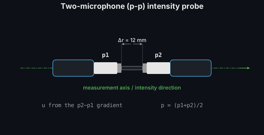
defeat the pressure methods. A p-p probe (see the
[Sound Intensity guide](https://jmrplens.github.io/phonometry/reference/api/power/intensity/)) is swept continuously over each of
`N` segments of a surface enclosing the source, reporting the segment-averaged
signed normal intensity ``.
The partial powers sum to the total:
$$
P_i = \langle I_{n,i} \rangle\ S_i, \qquad P = \sum_i P_i, \qquad
L_W = 10 \log_{10}\frac{P}{P_0},\quad P_0 = 1\ \text{pW} .
$$
[Watch the high-resolution video (WebM)](https://raw.githubusercontent.com/jmrplens/phonometry/main/.github/images/anim_intensity_scan_power.webm)
A band in which `P < 0` (net inflow, from a stronger source outside the
surface) is **not determinable** and reported as `NaN`. Two normative field
indicators qualify each band. The **surface pressure-intensity indicator**
`FpI` measures how reactive the field is, and the **negative-partial-power
indicator** `F+/-` measures how much energy circulates in and out:
$$
F_{pI} = [L_p] - L_W + 10 \log_{10}\frac{S}{S_0}, \qquad
F_{+/-} = 10 \log_{10}\frac{\sum_i \lvert P_i \rvert}{\lvert \sum_i P_i \rvert} .
$$
The probe's **dynamic capability** `Ld = δpI0 − K` (pressure-residual
intensity index minus the bias factor `K`, 10 dB for grade 2 and 7 dB for
grade 3) must exceed `FpI` (criterion 1); `F+/- ≤ 3 dB` is criterion 2
(mandatory for grade 2); and the two repeated sweeps must agree within the
Table 2 limit `s` per segment (criterion 3). A band is **engineering** grade
when criteria 1, 2 and 3 hold, **survey** when 1 and 3 hold, else `none`.
An A-weighted total additionally omits the bands failing criteria 1 and/or 2
(clause 10.6 b); the result flags them in `a_weighting_omitted_bands`.
```python
import numpy as np
from phonometry import emission
# 6 surface segments x 6 octave bands: signed normal intensity (W/m^2) from two
# repeated sweeps, the segment areas, and the per-segment surface SPL (dB).
freqs = np.array([125, 250, 500, 1000, 2000, 4000], dtype=float)
areas = np.full(6, 0.5) # 0.5 m^2 per segment
rng = np.random.default_rng(0)
scan1 = np.abs(rng.normal(1e-4, 2e-5, size=(6, 6))) # (segments, bands)
scan2 = scan1 * (1.0 + rng.normal(0.0, 0.02, size=(6, 6)))
pressure = np.full((6, 6), 80.0)
res = emission.sound_power_intensity(
scan1, areas, normal_intensity_2=scan2, pressure_levels=pressure,
pressure_residual_index=12.0, frequencies=freqs,
band_type="octave", grade="engineering",
)
print(np.round(res.sound_power_level, 1)) # per-band LW
print(round(res.sound_power_level_a, 1)) # LWA, determinable + qualified bands
print(round(float(res.dynamic_capability_index[0]), 1)) # Ld = 12 - 10 = 2.0 dB
print(round(float(res.surface_pressure_intensity_index[0]), 2)) # FpI
print(list(res.achieved_grade)) # per-band grade
res.plot() # LW spectrum; non-positive (undeterminable) bands hatched (needs matplotlib)
```
*The partial powers `·Si` of the six segments sum to each band's `LW`;
every band here nets positive power and passes the field-indicator criteria at
engineering grade, so all six bars stand, and the A-weighted total of
90.9 dB(A) heads the title.*
Show the code for this figure
```python
import matplotlib.pyplot as plt
import numpy as np
from phonometry import emission
# 6 surface segments x 6 octave bands: signed normal intensity (W/m^2) from two
# repeated sweeps, the segment areas, and the per-segment surface SPL (dB).
freqs = np.array([125, 250, 500, 1000, 2000, 4000], dtype=float)
areas = np.full(6, 0.5) # 0.5 m^2 per segment
rng = np.random.default_rng(0)
scan1 = np.abs(rng.normal(1e-4, 2e-5, size=(6, 6))) # (segments, bands)
scan2 = scan1 * (1.0 + rng.normal(0.0, 0.02, size=(6, 6)))
pressure = np.full((6, 6), 80.0)
res = emission.sound_power_intensity(
scan1, areas, normal_intensity_2=scan2, pressure_levels=pressure,
pressure_residual_index=12.0, frequencies=freqs,
band_type="octave", grade="engineering",
)
# res is the SoundPowerIntensityResult computed above. One line:
res.plot()
plt.show()
# By hand: a bar spectrum of LW with the A-weighted total in the title.
freqs = res.frequencies
positions = np.arange(freqs.size)
fig, ax = plt.subplots()
ax.bar(positions, res.sound_power_level, width=0.7, color="#1f77b4")
ax.set_xticks(positions)
ax.set_xticklabels([f"{f:g}" for f in freqs], rotation=45, ha="right")
ax.set_xlabel("Frequency [Hz]")
ax.set_ylabel("Sound power level LW [dB]")
ax.set_title(
f"Intensity-scanning sound power (ISO 9614-2) "
f"LWA = {res.sound_power_level_a:.1f} dB(A)")
plt.show()
```
Supplying `normal_intensity_2` (the second sweep) averages the two for the
partial powers and evaluates criterion 3; `pressure_levels` enables `FpI`;
`pressure_residual_index` (`δpI0`) plus a second sweep enables the per-band
achieved grade. The probe's finite-difference intensity has a
frequency-dependent bias handled in the [intensity guide](https://jmrplens.github.io/phonometry/reference/api/power/intensity/).
### `sound_power_intensity()` parameters
| Parameter | Type | Units | Range / default | Notes |
| :--- | :--- | :--- | :--- | :--- |
| `normal_intensity` | 2D array | W/m² | `(N_seg, N_bands)` | Signed segment-averaged normal intensity `` (first sweep) |
| `areas` | 1D array | m² | > 0, `(N_seg,)` | Segment areas `Si` |
| `normal_intensity_2` | 2D array | W/m² | same shape | Second sweep → criterion 3 and averaging |
| `pressure_levels` | 2D array | dB | same shape | Segment SPL `Lpi` → `FpI` |
| `pressure_residual_index` | float or 1D array | dB | — | `δpI0` → `Ld` / criterion 1 |
| `frequencies` | 1D array | Hz | nominal centres | `LWA` and Table 2 limits |
| `band_type` | str | — | `'third'` (default) / `'octave'` | Table 2 lookup |
| `grade` | str | — | `'engineering'` (default) / `'survey'` | Selects `K` |
| `repeatability_limit` | float or 1D array | dB | default Table 2 | Override criterion-3 `s` |
Returns a `SoundPowerIntensityResult`: `partial_power`/`partial_power_level`
per segment and band, `sound_power`/`sound_power_level` (band total, `NaN`
where `negative_band`), `surface_pressure_intensity_index` (`FpI`),
`negative_partial_power_index` (`F+/-`), `repeatability`,
`dynamic_capability_index` (`Ld`), `achieved_grade`, `surface_area`,
`sound_power_level_a` and `grade`.
## 4. Precision grade, anechoic room (ISO 3745)
When the highest accuracy is required, ISO 3745 measures sound power in a
qualified **anechoic** or **hemi-anechoic** room, where the free field lets a
fixed array of microphones sample the radiated sound pressure directly. It is the
grade-1 counterpart to the enveloping-surface method of Section 1, with
standardized microphone coordinates, a per-position background correction and an
explicit meteorological correction.
**Sound power level (Clause 8).** The band sound power level is the
surface-averaged pressure level plus the surface term and the corrections:
$$
L_W = \overline{L_p} + 10\lg\frac{S}{S_0} + C_1 + C_2 + C_3,
$$
with $S = 4\pi r^2$ over the sphere or $S = 2\pi r^2$ over the hemisphere,
$S_0 = 1\ \text{m}^2$. $C_1$ and $C_2$ are the meteorological corrections
(reference and radiation-impedance terms); $C_3$ accounts for air absorption over
the measurement radius. The microphone positions are the standardized
unit-vector arrays of Tables D.1 (sphere), E.1 (hemisphere) and E.2 (hemisphere,
broadband).
```python
import numpy as np
from phonometry import emission
# The 40 standardized hemisphere positions (unit vectors scaled by the radius).
pos = emission.precision_positions("hemisphere", radius=1.0, count=40)
print(pos.shape) # (40, 3)
# Octave/third-octave band SPL (dB) at each of the 40 positions; here a uniform
# 74 dB in one band. The result carries S = 2*pi*r^2 and LW with C1+C2+C3.
levels = np.full((40, 1), 74.0)
res = emission.sound_power_anechoic(levels, "hemisphere", radius=1.0)
print(round(res.surface_area, 3)) # 6.283 (2*pi*1^2)
print(np.round(res.sound_power_level, 2)) # [81.85]
```
**Background and meteorological corrections.** The $K_1$ background correction is
applied **per position** and floored where the signal-to-background difference is
small (Eq. 11); the meteorological correction is evaluated from the measured
temperature and static pressure.
```python
import numpy as np
from phonometry import emission
# K1 for a 6 dB signal-to-background difference in a <=200 Hz edge band: the
# floor is 1.26 dB (Eq. 11). Source and background levels are [positions, bands].
k1 = emission.precision_background_correction(
np.array([[56.0]]), np.array([[50.0]]), np.array([200.0]))
print(round(float(k1[0, 0]), 4)) # 1.2563
# Meteorological corrections at the 23 C, 101.325 kPa reference (Eq. 16):
mc = emission.meteorological_corrections(23.0, 101.325)
print(round(mc.c1, 4), round(mc.c2, 4)) # -0.1282 0.0
# Expanded uncertainty (Clause 10.5 EXAMPLE): sigma_R0 = 0.5, sigma_omc = 2.0,
# k = 2 -> U = 4.1 dB.
print(round(emission.precision_uncertainty(0.5, 2.0, 2.0), 3)) # 4.123
```
The `MeteorologicalCorrection` is a pair of scalars (plus the per-band `C3`
when the attenuation coefficient is supplied per band) rather than a
plottable spectrum: the corrections fold into the
`PrecisionSoundPowerResult` as its `c1`/`c2`/`c3` fields, and the `.report()`
fiche prints them on its measurement-basis strip.
Over several bands `sound_power_anechoic` returns a plottable
`PrecisionSoundPowerResult` carrying the per-band `LW` and the A-weighted total:
```python
import numpy as np
from phonometry import emission
# A mid-frequency-peaked machine measured over the 40-position hemisphere array
# (Annex E). levels_positions is the (40, NB) surface pressure spectrum: a base
# spectrum peaked near 1 kHz plus a small per-position spatial spread.
freqs = np.array([125, 250, 500, 1000, 2000, 4000, 8000], float)
base = 70.0 + 8.0 * np.exp(-(np.log2(freqs / 1000.0) ** 2) / 2.0)
rng = np.random.default_rng(7)
levels = base[None, :] + rng.normal(0.0, 1.0, (40, freqs.size))
result = emission.sound_power_anechoic(levels, "hemisphere", radius=1.0, frequencies=freqs)
print(round(result.sound_power_level_a, 1)) # 89.3
result.plot() # LW spectrum, LWA in the title (needs matplotlib)
```
*One bar per band: the surface-averaged pressure plus the area, background and
meteorological corrections give `LW(f)`, and the A-weighted energy sum across
bands gives the single-number `LWA` in the title.*
Show the code for this figure
```python
import matplotlib.pyplot as plt
import numpy as np
from phonometry import emission
# A mid-frequency-peaked machine measured over the 40-position hemisphere array
# (Annex E). levels_positions is the (40, NB) surface pressure spectrum: a base
# spectrum peaked near 1 kHz plus a small per-position spatial spread.
freqs = np.array([125, 250, 500, 1000, 2000, 4000, 8000], float)
base = 70.0 + 8.0 * np.exp(-(np.log2(freqs / 1000.0) ** 2) / 2.0)
rng = np.random.default_rng(7)
levels = base[None, :] + rng.normal(0.0, 1.0, (40, freqs.size))
result = emission.sound_power_anechoic(levels, "hemisphere", radius=1.0, frequencies=freqs)
# result is the PrecisionSoundPowerResult computed above. One line:
result.plot()
plt.show()
# By hand: a bar spectrum of LW with the A-weighted total in the title.
freqs = result.frequencies
positions = np.arange(freqs.size)
fig, ax = plt.subplots()
ax.bar(positions, result.sound_power_level, width=0.7, color="#1f77b4")
ax.set_xticks(positions)
ax.set_xticklabels([f"{f:g}" for f in freqs], rotation=45, ha="right")
ax.set_xlabel("Frequency [Hz]")
ax.set_ylabel("Sound power level LW [dB]")
ax.set_title(
f"Precision sound power (ISO 3745) LWA = {result.sound_power_level_a:.1f} dB(A)")
plt.show()
```
## 5. Precision intensity scanning (ISO 9614-3)
ISO 9614-3 is the grade-1 scanning method: like ISO 9614-2 it integrates the
normal intensity over a surface enclosing the source, but with a continuous
scan, tighter field-indicator criteria and an explicit uncertainty budget.
**Power and level (Clause 7).** The partial power of each segment is
$P_i = I_{n,i}\,S_i$; the total $P = \sum_i P_i$ gives
$L_W = 10\lg(P/P_0)$, $P_0 = 1\ \text{pW}$. A band whose net intensity is
negative (more power flowing in than out) is flagged not-applicable rather than
logged. The field indicators (temporal variability $F_T$, the signed and
unsigned pressure–intensity indicators, and the non-uniformity $F_S$) drive the
five acceptance criteria.
```python
import numpy as np
from phonometry import emission
# A fully enclosing surface with a uniform normal intensity In = W/S recovers
# the source power exactly: LW = 10*lg(W/P0). Here W = 100 uW -> 80 dB.
areas = np.array([0.5, 1.0, 0.25, 2.0])
w = 1.0e-4
i_n = np.full(areas.shape, w / float(areas.sum()))
res = emission.sound_power_intensity_precision(i_n, areas)
print(round(float(res.sound_power[0]), 6)) # 0.0001
print(round(float(res.sound_power_level[0]), 2)) # 80.0
```
Across several bands the result carries the per-band `LW` (`NaN` where the net
power is non-positive), flags those bands `not_applicable`, and draws them
with the one-line `result.plot()` of the figure below:
```python
import numpy as np
from phonometry import emission
# Four partial surfaces scanned over five one-third-octave bands. Each cell of
# partial_intensity is the signed normal intensity In_i (W/m^2); areas are the
# partial-surface areas Si. The 250 Hz band has net-negative power (a locally
# reactive field), so ISO 9614-3 flags it not-applicable (clause 9.2) -> NaN.
freqs = np.array([250, 500, 1000, 2000, 4000], float)
areas = np.array([0.5, 1.0, 0.75, 0.5])
base_intensity = np.array([2.0e-6, 8.0e-6, 2.0e-5, 1.0e-5, 3.0e-6])
partial_intensity = base_intensity[None, :] * np.array([1.0, 1.1, 0.9, 1.05])[:, None]
partial_intensity[:, 0] = [2.0e-6, -3.0e-6, -4.0e-6, -1.0e-6] # net-negative band
result = emission.sound_power_intensity_precision(partial_intensity, areas, frequencies=freqs)
print(result.not_applicable_band.tolist()) # [True, False, False, False, False]
print(round(result.sound_power_level_a, 1)) # 80.6
result.plot() # LW spectrum; the not-applicable band is hatched (needs matplotlib)
```
*The 250 Hz band nets negative (more energy flowing in than out), so ISO 9614-3
declares it not-applicable; the figure hatches and greys it while the four
determinate bands and the A-weighted total stand.*
Show the code for this figure
```python
import matplotlib.pyplot as plt
import numpy as np
from phonometry import emission
# Four partial surfaces scanned over five one-third-octave bands. Each cell of
# partial_intensity is the signed normal intensity In_i (W/m^2); areas are the
# partial-surface areas Si. The 250 Hz band has net-negative power (a locally
# reactive field), so ISO 9614-3 flags it not-applicable (clause 9.2) -> NaN.
freqs = np.array([250, 500, 1000, 2000, 4000], float)
areas = np.array([0.5, 1.0, 0.75, 0.5])
base_intensity = np.array([2.0e-6, 8.0e-6, 2.0e-5, 1.0e-5, 3.0e-6])
partial_intensity = base_intensity[None, :] * np.array([1.0, 1.1, 0.9, 1.05])[:, None]
partial_intensity[:, 0] = [2.0e-6, -3.0e-6, -4.0e-6, -1.0e-6] # net-negative band
result = emission.sound_power_intensity_precision(partial_intensity, areas, frequencies=freqs)
# result is the PrecisionIntensityResult computed above. One line:
result.plot()
plt.show()
# By hand: determinate bands as LW bars; a not-applicable band (its LW is NaN)
# is flagged by a full-height greyed, hatched span rather than a zero-height bar.
freqs = result.frequencies
positions = np.arange(freqs.size)
neg = result.not_applicable_band
lw = np.nan_to_num(result.sound_power_level)
fig, ax = plt.subplots()
ax.bar(positions[~neg], lw[~neg], width=0.7, color="#1f77b4")
for pos in positions[neg]:
ax.axvspan(pos - 0.35, pos + 0.35, facecolor="#888888", alpha=0.28,
hatch="//", edgecolor="#888888")
ax.set_xticks(positions)
ax.set_xticklabels([f"{f:g}" for f in freqs], rotation=45, ha="right")
ax.set_xlabel("Frequency [Hz]")
ax.set_ylabel("Sound power level LW [dB]")
ax.set_title(
f"Precision intensity scanning (ISO 9614-3) "
f"LWA = {result.sound_power_level_a:.1f} dB(A)")
plt.show()
```
## 6. The measurement report (`.report()`)
A sound power determination ends as a *document*. Every result of this page
stays plottable while it is being worked on — `res.plot()` draws the same
`LW` spectrum interactively that the fiche typesets — and the report step
wraps it into the deliverable. Both the enveloping-surface result
(`SoundPowerResult`, ISO 3744/3746) and the precision result
(`PrecisionSoundPowerResult`, ISO 3745) expose a `.report()` method that writes
a one-page PDF fiche laid out like a sound-power test sheet: the standard-basis
line naming the applied method and accuracy grade, an optional metadata header
(client, noise source, test environment, instrumentation, climate, date), a
per-band table (nominal octave/one-third-octave frequency, the surface
sound-pressure level `Lp` and the band sound-power level `LW`), the
sound-power spectrum `LW(f)` with a nominal band axis, and a boxed A-weighted
sound power level `LWA` (dB re 1 pW) with the total `LW`, the expanded
uncertainty `U` and the measurement surface area `S` alongside.
The metadata is supplied through a `ReportMetadata`, whose applicable fields
here are the **source description** (`specimen`), the **test environment**
(`test_room`), the **client**, the **instrumentation**, the **temperature**,
**relative humidity** and **ambient pressure**, the **date of test**
(`test_date`) and the footer identity (`laboratory`, `operator`, `report_id`,
`notes`); the measurement surface area `S` comes from the result itself and is
printed in the result box and the basis strip, together with the applied
corrections (the background `K1` and environmental `K2` for the ISO 3744/3746
surface method, or the meteorological `C1`/`C2`/`C3` for the ISO 3745
precision method). Supplying `requirement` adds a PASS/FAIL verdict against a
declared A-weighted sound-power limit (a sound-power emission is a quantity where
less is better, so the source passes at or below the limit). `verbose=True`
adds the energy-averaged level `Lp'` to the table, and for the ISO 3744/3746
surface result it also adds the `K1`/`K2` correction columns (the ISO 3745
precision result carries no `K1`/`K2`; its `C1`/`C2`/`C3` appear in the
basis strip). `language="es"` renders the Spanish fiche with comma decimals.
```python
import numpy as np
from phonometry import ReportMetadata, emission
freqs = np.array([63, 125, 250, 500, 1000, 2000, 4000, 8000], float)
# Ten identical position spectra over a hemisphere of radius 4 m; background a
# uniform 10 dB below and an equivalent absorption area A = 1500 m^2 (so K1, K2
# are meaningful and within the engineering validity limit).
surface = np.array([72.0, 76, 80, 82, 81, 78, 73, 66])
res = emission.sound_power_pressure(
np.tile(surface, (10, 1)), "hemisphere", radius=4.0,
background_levels=np.tile(surface - 10.0, (10, 1)),
frequencies=freqs, absorption_area=1500.0, grade="engineering",
)
res.report(
"sound_power.pdf",
metadata=ReportMetadata(
client="Example manufacturing plant",
specimen="Hydraulic power pack (floor-standing)",
test_room="Hemi-anechoic room over a reflecting floor",
instrumentation="Class 1 sound level meter (IEC 61672-1), s/n 0042",
laboratory="Phonometry reference example",
report_id="EXAMPLE-3744",
requirement=105.0,
),
) # LWA = 103.7 dB(A) re 1 pW -> declared limit 105 dB(A): PASS
```
The example fiche, regenerated with `make reports`, is kept rendered in the
repository. Click the preview to open the PDF:
[](https://raw.githubusercontent.com/jmrplens/phonometry/main/.github/reports/iso3744_sound_power_example.pdf)
*Sound power determination fiche (`SoundPowerResult.report`), an ISO 3744
engineering-grade hemisphere measurement with the K1/K2 corrections and the
boxed LWA.*
### The intensity determination (ISO 9614-2)
The intensity-scanning result (`SoundPowerIntensityResult`, ISO 9614-2) writes
the same one-page fiche through its own `.report()`. The standard-basis line
names ISO 9614-2:1996 and the measurement grade, the per-band table lists the
intensity-derived band sound-power level `LW`, and the boxed `LWA` carries
the total `LW`, the measurement surface `S` and the determination grade
(the intensity result has no expanded uncertainty `U`). `verbose=True` adds the
field indicators `FpI` (surface pressure-intensity) and `F+/-`
(negative partial power) and the per-band achieved grade; the basis strip
states the partial-power model (the segment partial powers `Pi = In,i·Si`
summing to `P`) and the Annex B qualification criteria. A band whose net power
is non-positive is not determinable (clause 9.2) and prints an em dash.
```python
import numpy as np
from phonometry import ReportMetadata, emission
freqs = np.array([125, 250, 500, 1000, 2000, 4000], float)
# Six equal 0.5 m^2 segments (S = 3.0 m^2); one uniform normal-intensity
# spectrum scanned twice, with the surface SPL and the instrument residual
# index that qualify every band at engineering grade.
intensity = np.array([0.6e-4, 1.0e-4, 1.5e-4, 1.4e-4, 0.9e-4, 0.5e-4])
scan = np.tile(intensity, (6, 1))
res = emission.sound_power_intensity(
scan, np.full(6, 0.5), normal_intensity_2=scan.copy(),
pressure_levels=np.full((6, 6), 80.0), pressure_residual_index=15.0,
frequencies=freqs, band_type="octave", grade="engineering",
)
res.report(
"sound_power_intensity.pdf",
metadata=ReportMetadata(
client="Example manufacturing plant",
specimen="Hydraulic power pack (floor-standing)",
test_room="Machine hall with steady background noise",
instrumentation="Class 1 p-p intensity probe (IEC 61043), s/n 0042",
laboratory="Phonometry reference example",
report_id="EXAMPLE-9614",
requirement=93.0,
),
) # LWA = 90.9 dB(A) re 1 pW -> declared limit 93 dB(A): PASS
```
The example fiche, regenerated with `make reports`, is kept rendered in the
repository. Click the preview to open the PDF:
[](https://raw.githubusercontent.com/jmrplens/phonometry/main/.github/reports/iso9614_sound_power_intensity_example.pdf)
*Sound power by intensity fiche (`SoundPowerIntensityResult.report`), an
ISO 9614-2 engineering-grade scan with the field indicators and the boxed
LWA.*
### The reverberation-room determination (ISO 3741)
The reverberation-room result (`ReverberationSoundPowerResult`, ISO 3741) writes
the same one-page fiche through its own `.report()`. The standard-basis line
names ISO 3741:2010 and the precision accuracy grade (grade 1) and states which
method was used, the direct method using the room equivalent absorption area
(Eq. 20) or the comparison method using a reference sound source (Eq. 21). The
per-band table lists the mean room sound-pressure level `Lp` and the band
sound-power level `LW`, and the boxed `LWA` carries the total `LW` and the
determination method (the reverberation result has no expanded uncertainty `U`).
`verbose=True` adds the background correction `K1` and, for the direct method,
the equivalent absorption area `A` and the Waterhouse boundary correction `Cw`;
the basis strip states the correction model (Eq. 20 or Eq. 21), the applied
meteorological corrections `C1`/`C2` and the speed of sound, and cites the
Annex F A-weighting.
```python
import numpy as np
from phonometry import ReportMetadata, emission
freqs = np.array([125, 250, 500, 1000, 2000, 4000, 8000], float)
# Octave-band mean room sound-pressure levels in a qualified
# reverberation room of V = 200 m3, S = 240 m2, with a uniform T60 = 2.0 s.
lp = np.array([80.0, 83.0, 85.0, 84.0, 80.0, 75.0, 68.0])
res = emission.sound_power_reverberation(
lp, 2.0, volume=200.0, surface_area=240.0, frequencies=freqs,
temperature=20.0, static_pressure=101.325,
)
res.report(
"sound_power_reverberation.pdf",
metadata=ReportMetadata(
client="Example manufacturing plant",
specimen="Hydraulic power pack (floor-standing)",
test_room="Qualified reverberation room, V = 200 m3, T60 = 2.0 s",
instrumentation="Class 1 sound level meter (IEC 61672-1), s/n 0042",
laboratory="Phonometry reference example",
report_id="EXAMPLE-3741",
requirement=96.0,
),
) # LWA = 94.3 dB(A) re 1 pW -> declared limit 96 dB(A): PASS
```
The example fiche, regenerated with `make reports`, is kept rendered in the
repository. Click the preview to open the PDF:
[](https://raw.githubusercontent.com/jmrplens/phonometry/main/.github/reports/iso3741_reverberation_power_example.pdf)
*Reverberation-room sound power fiche (`ReverberationSoundPowerResult.report`),
an ISO 3741 precision-grade direct-method determination with the Waterhouse and
C1/C2 corrections and the boxed LWA.*
## 7. Declaring the noise emission (ISO 4871)
A measured sound power level is not yet a *declaration*. ISO 4871:1996 is the
standard for the noise-emission declaration a manufacturer prints in technical
documents: which quantities are stated, in which form, and how a declared value
is verified. The preferred quantity is the A-weighted sound power level
`L_WA`, optionally accompanied by the A-weighted emission sound pressure level
`L_pA` at a work station.
A declaration takes one of two alternative forms (clause 4):
- the **dual-number** form (clause 3.16): the measured value `L_WA` and its
uncertainty `K_WA` stated together but separately; and
- the **single-number** form (clause 3.15): the derived declared value
`L_WAd = L_WA + K_WA`, an upper limit that repeated measurements are unlikely
to exceed at the stated confidence level.
`K_WA` combines the measurement (reproducibility) and, for a batch, the
production spread; for a single machine `K = 1.645 sigma_R` (Annex A.2.2). A
`NoiseEmissionDeclaration` holds one or more per-operating-mode declarations
and renders the ISO 4871 fiche through `.report()`. The quickest route is to
`declare()` straight from a measured sound power:
```python
import numpy as np
import phonometry as ph
from phonometry import ReportMetadata
# ... a measured LWA from ISO 3744 ...
result = ph.sound_power_pressure(levels, "hemisphere", radius=1.0,
frequencies=freqs)
declaration = result.declare(
uncertainty=2.0, # K_WA in dB (defaults to the expanded U)
machine="Type 990, Model 11-TC",
operating_conditions="50 Hz, 230 V, rated load",
basic_standards="ISO 3744",
verification_level=result.sound_power_level_a, # L_1 for clause 6.2
)
declaration.report(
"iso4871.pdf",
metadata=ReportMetadata(measurement_standard="ISO 3744"),
) # -> L_WAd = L_WA + K_WA, verified when L_1 <= L_WAd
```
Or build the declaration directly, reproducing the ISO 4871 Annex B example
(two operating modes, `L_WA = 88` and `95` dB with `K_WA = 2` dB, giving
declared `L_WAd = 90` and `97` dB):
```python
mode1 = ph.OperatingModeDeclaration(
"Operating mode 1", sound_power_level=88.0, sound_power_uncertainty=2.0,
emission_pressure_level=78.0, emission_pressure_uncertainty=2.0,
verification_level=89.0, # passes: 89 <= 90
)
mode2 = ph.OperatingModeDeclaration(
"Operating mode 2", sound_power_level=95.0, sound_power_uncertainty=2.0,
emission_pressure_level=86.0, emission_pressure_uncertainty=2.0,
verification_level=98.0, # fails: 98 > 97
)
ph.NoiseEmissionDeclaration(
(mode1, mode2), machine="Type 990, Model 11-TC",
basic_standards=("ISO 3744", "ISO 11202"), form="dual-number",
).report("iso4871.pdf")
```
The example fiche, regenerated with `make reports`, is kept rendered in the
repository. Click the preview to open the PDF:
[](https://raw.githubusercontent.com/jmrplens/phonometry/main/.github/reports/iso4871_declaration_example.pdf)
*Noise emission declaration fiche (`NoiseEmissionDeclaration.report`), the
ISO 4871 Annex B dual-number table with the declared `L_WAd = L_WA + K_WA` and
the clause 6.2 verification verdict.*
## See also
- [Sound Intensity (p-p)](https://jmrplens.github.io/phonometry/reference/api/power/intensity/): the two-microphone probe, its
finite-difference bias and the ISO 9614-1 field indicators behind the
scanning method.
- [Room Acoustics](https://jmrplens.github.io/phonometry/reference/api/rooms/room-acoustics/): the reverberation time
and equivalent absorption area (ISO 354) that feed `K2` and the ISO 3741
absorption area; impact and airborne insulation.
- [Levels](https://jmrplens.github.io/phonometry/reference/api/levels/levels/): energy averaging and the A-weighting behind `LWA`.
- [Theory](https://jmrplens.github.io/phonometry/reference/theory/environment-transport/): the Waterhouse, K1/K2 and C1/C2 derivations.
- API reference: [`emission.sound_power`](https://jmrplens.github.io/phonometry/reference/api/power/sound-power/), [`emission.sound_power_reverberation`](https://jmrplens.github.io/phonometry/reference/api/power/sound-power-reverberation/) and [`emission.sound_power_intensity`](https://jmrplens.github.io/phonometry/reference/api/power/sound-power-intensity/).
## Quick answers
### What is the difference between sound power and sound pressure?
Sound pressure depends on where you stand and on the room; sound power does
not. The sound power level `LW` is the total acoustic energy per second a
source radiates, referenced to `P0 = 1 pW`, and it is the device-independent
emission descriptor that goes on a datasheet or is checked against a
noise-emission limit; ISO 3744, ISO 3741, ISO 9614-2, ISO 3745 and
ISO 9614-3 all determine it.
### What do the accuracy grades in sound power measurement mean?
The grade is a claim about reproducibility: `σR0` is the standard deviation
you would see if different laboratories measured the same source, each
following the standard correctly. Typical A-weighted values are
`σR0 ≈ 0.5 dB` for grade 1 (ISO 3741), `1.5 dB` for grade 2 (ISO 3744,
ISO 9614-2) and `3 dB` or more for grade 3. A grade-2 `LWA` carries
`U ≈ 3 dB`, so two grade-2 results 2 dB apart are statistically
indistinguishable.
### How do I measure sound power when background noise cannot be switched off?
Use intensity scanning: ISO 9614-2 (grade 2 or 3) or ISO 9614-3 (grade 1,
precision). Because sound intensity is the net energy flux through the
measurement surface, steady extraneous noise even some 10 dB above the
source is tolerated, whereas the ISO 3744 pressure method needs the
background at least 6 dB below the source. The per-band field indicators
then decide the grade actually achieved.
## References
- Fahy, F. J. (1995). *Sound intensity* (2nd ed.). E&FN Spon.
ISBN 978-0-419-19810-9.
[doi:10.4324/9780203475386](https://doi.org/10.4324/9780203475386).
The monograph on sound energy flux: why intensity separates the energy
leaving the source from steady energy passing through, behind the
scanning methods of sections 3 and 5.
- Beranek, L. L., & Mellow, T. J. (2012). *Acoustics: Sound fields and
transducers*. Academic Press. ISBN 978-0-12-391421-7.
[doi:10.1016/C2011-0-05897-0](https://doi.org/10.1016/C2011-0-05897-0).
Radiation and sound fields: the free-field and diffuse-field relations
between pressure and power that the enveloping-surface and
reverberation-room methods rest on.
- International Organization for Standardization. (2019). *Acoustics —
Determination of sound power levels of noise sources — Guidelines for the
use of basic standards* (ISO 3740:2019).
[iso.org catalogue](https://www.iso.org/standard/45107.html).
The selection guide behind "Choosing a method": grades, environments,
source-size and background criteria for the whole family.
- International Organization for Standardization. (2010). *Acoustics —
Determination of sound power levels and sound energy levels of noise
sources using sound pressure — Precision methods for reverberation test
rooms* (ISO 3741:2010).
[iso.org catalogue](https://www.iso.org/standard/52053.html).
The reverberation-room method of section 2.
- International Organization for Standardization. (2010). *Acoustics —
Determination of sound power levels and sound energy levels of noise
sources using sound pressure — Engineering methods for an essentially free
field over a reflecting plane* (ISO 3744:2010).
[iso.org catalogue](https://www.iso.org/standard/52055.html).
The enveloping-surface method of section 1.
- International Organization for Standardization. (2012). *Acoustics —
Determination of sound power levels and sound energy levels of noise
sources using sound pressure — Precision methods for anechoic rooms and
hemi-anechoic rooms* (ISO 3745:2012).
[iso.org catalogue](https://www.iso.org/standard/45362.html).
The precision anechoic-room method of section 4.
- International Organization for Standardization. (1996). *Acoustics —
Declaration and verification of noise emission values of machinery and
equipment* (ISO 4871:1996).
[iso.org catalogue](https://www.iso.org/standard/10868.html).
The declaration behind section 7: the dual/single-number forms,
`L_WAd = L_WA + K_WA` (clause 3.15) and the clause 6.2 verification.
## Standards
ISO 3744:2010, *Acoustics — Determination of sound power levels
and sound energy levels of noise sources using sound pressure — Engineering
methods for an essentially free field over a reflecting plane*: the
enveloping-surface method: hemisphere and box surface areas, the `K1`/`K2`
corrections, the Annex B microphone positions and the Annex E A-weighting.
ISO 3746:2010, *… Survey method using an enveloping measurement surface over a
reflecting plane*: the survey grade sharing the same formulae with coarser
criteria. ISO 3741:2010, *… Precision methods for reverberation test rooms*:
the direct (Eq. 20) and comparison methods with the Waterhouse and
meteorological corrections and the Table 1 qualification criteria.
ISO 3745:2012, *… Precision methods for anechoic rooms and hemi-anechoic
rooms*: the Clause 8 power level, the per-position background correction
(Eq. 11), the meteorological corrections and the standardized microphone
arrays. ISO 9614-2:1996, *Acoustics — Determination of sound power levels of
noise sources using sound intensity — Part 2: Measurement by scanning* — the
partial powers, the `FpI` and `F+/-` field indicators and the grade criteria.
ISO 9614-3:2002, *… Part 3: Precision method for measurement by scanning*:
the grade-1 scanning method, its field indicators and the clause 9.2
not-applicable flagging. ISO 4871:1996, *Acoustics — Declaration and
verification of noise emission values of machinery and equipment*: the
dual-number and single-number declaration forms, the declared value
`L_WAd = L_WA + K_WA` and the clause 6.2 verification of section 7.