Source: https://jmrplens.github.io/phonometry/guides/sections/room-acoustics/ # Room Acoustics Room acoustics starts from one measurement: the **impulse response** (IR) between a source and a receiver. Filter it into bands and integrate it, and it yields reverberation time, clarity and speech intelligibility: everything about the sound field inside a single room. This page follows that chain in measurement order: acquiring the IR (ISO 18233), turning it into room parameters (ISO 3382-1/2), spatial speech metrics for open-plan offices (ISO 3382-3) and, closing the loop, the sound absorption of a material in a reverberation room (ISO 354). For sound insulation *between* spaces (the same IR measured either side of a partition) see the companion [Field Insulation Measurement and Ratings guide](https://jmrplens.github.io/phonometry/guides/insulation-field/). ## 1. Impulse-response acquisition (ISO 18233) A room behaves, to a good approximation, as a **linear time-invariant** system, so everything about it is contained in its IR. You could fire a pistol and record the tail, but a deterministic excitation played through a loudspeaker and *deconvolved* recovers the same IR with 20–30 dB more effective signal-to-noise ratio (ISO 18233). Two excitations are provided. **Exponential sine sweep (ESS, Annex B).** The instantaneous frequency rises exponentially, $$ f(t) = f_1 \left( \frac{f_2}{f_1} \right)^{t/T}, $$ so the time spent per octave is constant and the excitation mimics pink noise (constant energy per fractional-octave band). The IR is recovered by linear (zero-padded, non-circular) spectral division, $$ H = \frac{Y\ \overline{X}}{|X|^2 + \varepsilon}, $$ with a small Tikhonov term $\varepsilon$ guarding the band edges where the sweep has little energy. Because a low-to-high sweep places harmonic distortion at *negative* arrival times, distortion separates cleanly from the linear IR and is discarded by keeping only the causal part. The `"farina"` method reaches the same result by convolving the recording with the analytic inverse filter; it assumes the reference sweep was generated with the default amplitude and fade, so use the spectral method for a non-unit-amplitude or custom-fade sweep. **Maximum-length sequence (MLS, Annex A).** An order-`N` binary sequence of length $2^N-1$ whose circular autocorrelation is a near-perfect delta; the IR follows from circular cross-correlation of the recorded period with the sequence. MLS excites at constant amplitude and is quick to average, but it is more sensitive to time variance (draughts, temperature drift) and cannot be fed as much power as a sweep. **Prefer the sweep** for rooms and partitions; reach for MLS when the excitation must be periodic or the hardware favours a two-level signal. ```python import numpy as np from scipy.signal import fftconvolve from phonometry import room fs = 48000 # A 3 s, 20 Hz - 20 kHz sweep is a good broadband room excitation # sweep: excitation you play through the loudspeaker sweep = room.sweep_signal(fs, 20.0, 20000.0, 3.0) # Deconvolve the recorded response back to the impulse response system = np.zeros(fs); system[100] = 1.0; system[2000] = 0.4 # direct + reflection # recorded: mic capture of the played sweep (here simulated by convolution with a synthetic room) recorded = fftconvolve(sweep, system) ir = room.impulse_response(recorded, sweep, fs, method="spectral") print(int(np.argmax(np.abs(ir)))) # 100: direct sound recovered ir.plot() # waveform + Schroeder envelope (figure below) # Farina inverse-filter variant (needs the sweep band) ir_f = room.impulse_response(recorded, sweep, fs, method="farina", f_range=(20.0, 20000.0)) # Periodic MLS: excite with >= 2 periods, average, cross-correlate mls = room.mls_signal(16) # length 2**16 - 1 = 65535 rec = fftconvolve(np.tile(mls, 2), system)[: 2 * mls.size] ir_m = room.mls_impulse_response(rec, mls) print(int(np.argmax(np.abs(ir_m)))) # 100 ``` `sweep_signal`/`mls_signal` return plain arrays, ready to write to a WAV file and play. `impulse_response`/`mls_impulse_response` return an `ImpulseResponseResult`, a drop-in for the raw IR array (`np.asarray(ir)`, indexing and `ir.size` all keep working, so `room_parameters(ir, fs)` is unchanged) that also carries the sample rate and method and adds an `.plot()`. Two more excitations from the transfer-function literature - complementary Golay pairs with exactly noise-free deconvolution, and sweeps shaped to an arbitrary target spectrum - live in the [system-measurement guide](https://jmrplens.github.io/phonometry/guides/system-measurement/) and return the same result types. **The two excitations.** The exponential sweep sweeps its energy up the spectrum over the whole signal, while the MLS is a flat-spectrum two-level sequence, visible as the near-constant magnitude on the right.

Show the code for this figure

```python from phonometry import room from phonometry import plot_excitation fs = 48000 sweep = room.sweep_signal(fs, 50.0, 20000.0, 1.0) # ESS excitation mls = room.mls_signal(12).astype(float) # length 2**12 - 1 # One-liner: waveform + spectrogram (sweep), sequence + flat spectrum (MLS) plot_excitation(sweep, fs, kind="sweep") plot_excitation(mls, fs, kind="mls") # By hand: the sweep spectrogram and the MLS magnitude spectrum import numpy as np import matplotlib.pyplot as plt fig, (ax1, ax2) = plt.subplots(1, 2, figsize=(12, 4)) ax1.specgram(sweep, NFFT=1024, Fs=fs, noverlap=512) ax1.set(xlabel="Time [s]", ylabel="Frequency [Hz]", title="Sweep spectrogram") spec = np.abs(np.fft.rfft(mls)) freqs = np.fft.rfftfreq(mls.size, d=1.0 / fs) ax2.semilogx(freqs[1:], 20 * np.log10(spec[1:] / np.median(spec[1:]))) ax2.set(xlabel="Frequency [Hz]", ylabel="Magnitude [dB]", title="MLS spectrum (flat)") ```

**The recovered impulse response.** Deconvolving the recording gives the broadband IR: the direct sound, discrete early reflections and the decaying diffuse tail. Its `.plot()` shows the waveform above and the log-magnitude envelope with the Schroeder energy-decay curve below: the straight decay whose slope becomes the reverberation time in §2. [Watch the high-resolution video (WebM)](https://raw.githubusercontent.com/jmrplens/phonometry/main/.github/images/anim_sweep_deconvolution.webm)

Show the code for this figure

```python import numpy as np from scipy.signal import fftconvolve from phonometry import room fs = 48000 sweep = room.sweep_signal(fs, 20.0, 20000.0, 1.5) # A synthetic room: direct sound + two reflections + a decaying diffuse tail system = np.zeros(int(0.7 * fs)) system[80], system[1400], system[3100] = 1.0, 0.5, 0.32 ir = room.impulse_response(fftconvolve(sweep, system), sweep, fs, length=system.size) # One-liner: waveform + log-magnitude / Schroeder decay ir.plot() # By hand: the normalized log-magnitude envelope in dB import matplotlib.pyplot as plt h = np.asarray(ir) t = np.arange(h.size) / fs plt.plot(t, 20 * np.log10(np.abs(h) / np.max(np.abs(h)))) plt.ylim(-80, 5) plt.xlabel("Time [s]"); plt.ylabel("Level re peak [dB]") ```

**Where to measure.** One IR characterises a single source–receiver pair; a reported room parameter is the spatial average over several. ISO 3382-1 (performance spaces) asks for at least two source positions and microphones spaced $\geq 2$ m apart, $\geq 1$ m from any surface, at $1.2$ m (seated-ear) height; ISO 3382-2 fixes the minimum number of source, microphone and source–microphone combinations per accuracy grade (survey / engineering / precision) and asks for microphone positions that avoid symmetric placements. **Averaging across positions.** The reported per-band parameter is the arithmetic mean over all source-microphone combinations, and the spread across positions is part of the answer, not noise: quote it alongside the mean whenever it exceeds the parameter's JND (§2), because a room can meet a target on average while individual seats sit far outside it. Four placement mistakes bias the mean itself: - **Correlated positions.** Microphones closer than 2 m to each other sample nearly the same sound field twice, so the average looks more stable than it is. The 1 m minimum from any surface likewise avoids the pressure build-up near a boundary (and the comb filter of the animation below) that colours everything a too-close microphone records. [Watch the high-resolution video (WebM)](https://raw.githubusercontent.com/jmrplens/phonometry/main/.github/images/anim_comb_filtering.webm) - **Symmetric placements.** In a geometrically symmetric room, mirror-image positions receive mirror-image reflection patterns; averaging them adds no new information. This is why ISO 3382-2 asks for positions that do not sit on symmetry lines. - **Too close to the source.** Inside the direct field EDT collapses and C80 saturates upward no matter what the room does. ISO 3382-2 therefore keeps every microphone at least $d_{min} = 2\sqrt{V/(c\,\hat T)}$ from the source, with $\hat T$ an estimate of the expected reverberation time (about 2.2 m for a 200 m³ classroom with an expected 0.5 s). - **Low-frequency luck.** Below the Schroeder frequency (§2) each band holds only a handful of room modes, and a microphone on a node of one of them sees a different decay than a microphone on an antinode. The spread of the 63-125 Hz bands across positions is structurally larger; the cure is more positions, not a longer excitation. ### `sweep_signal()` / `inverse_filter()` parameters | Parameter | Type | Units | Range / default | Notes | | :--- | :--- | :--- | :--- | :--- | | `fs` | int | Hz | > 0 | Sampling frequency | | `f1` | float | Hz | > 0, at/below lowest band | Sweep start frequency | | `f2` | float | Hz | `f1 < f2 <= fs/2` | Sweep stop frequency | | `seconds` | float | s | any; longer ⇒ more SNR | Sweep duration | | `amplitude` | float | — | default `1.0` | Peak amplitude | | `fade` | float | — | `[0, 0.5)`, default `0.01` | Half-Hann fade fraction (kills start/stop transients) | ### `impulse_response()` parameters | Parameter | Type | Units | Range / default | Notes | | :--- | :--- | :--- | :--- | :--- | | `recorded` | 1D array | any | non-empty | Recorded system response | | `reference` | 1D array | any | non-empty | The emitted sweep | | `fs` | int | Hz | > 0 | Sample rate | | `method` | str | — | `'spectral'` (default) / `'farina'` | `'farina'` requires `f_range` | | `f_range` | (float, float) | Hz | default `None` | `(f1, f2)` of the sweep (Farina only) | | `regularization` | float | — | default `1e-6` | Tikhonov term as a fraction of peak spectral energy | | `length` | int, optional | samples | default `len(recorded)` | Samples of causal IR to return | | `return_full` | bool | — | default `False` | Return the full sequence (distortion in the tail) | `mls_signal(order)` takes an integer `order` in 2–20 (sequence length $2^{\text{order}}-1$); `mls_impulse_response(recorded, mls, length=None)` needs `recorded` to span an integer number of MLS periods. ## 2. 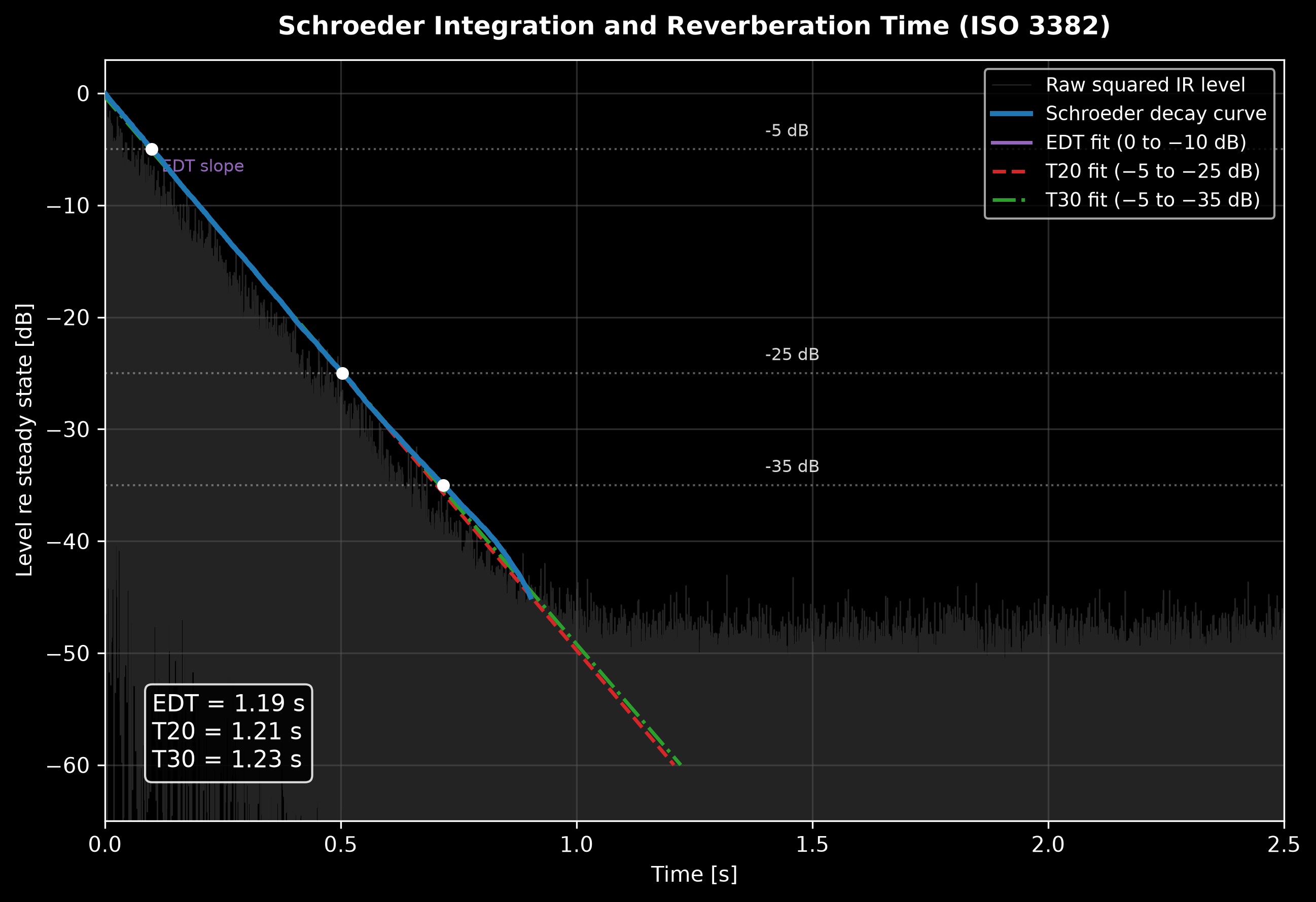Decay analysis and room parameters (ISO 3382-1/2) The IR is filtered into octave (or one-third-octave) bands and each band is turned into a **decay curve** by Schroeder backward integration of the squared IR: $$ E(t) = \int_t^{\infty} p^2(\tau)\ d\tau, \qquad L(t) = 10 \log_{10} \frac{E(t)}{E(0)}\ \text{dB}. $$ Integrating *backwards* removes the fluctuation that plagues a raw squared IR and yields a smooth curve whose slope is the decay rate. Background noise would make $E(t)$ level off, so integration is truncated where the fitted decay line crosses the noise floor and the missing tail is compensated assuming an exponential decay. Reverberation times come from a least-squares line fit over an evaluation range, extrapolated to a full 60 dB drop, $T = -60/\text{slope}$: **EDT** over 0 to −10 dB (perceived reverberance), **T20** over −5 to −25 dB and **T30** over −5 to −35 dB. Energy splits at an early/late boundary give **clarity** and **definition**, $$ C_{te} = 10 \log_{10} \frac{\int_0^{te} p^2\ dt}{\int_{te}^{\infty} p^2\ dt}\ \text{dB}, \qquad D_{50} = \frac{\int_0^{0.05} p^2\ dt}{\int_0^{\infty} p^2\ dt}, $$ with $te = 50$ ms → C50 (speech) and $te = 80$ ms → C80 (music), plus the **centre time** $T_s = \int t\ p^2\ dt / \int p^2\ dt$. Each parameter has a **just-noticeable difference** (ISO 3382-1 Table A.1: EDT 5 %, C80 1 dB, D50 0.05, Ts 10 ms) that sets how precisely it is worth reporting. [Watch the high-resolution video (WebM)](https://raw.githubusercontent.com/jmrplens/phonometry/main/.github/images/anim_schroeder.webm) *The jagged squared IR (grey) integrates to the smooth Schroeder curve (blue); the EDT, T20 and T30 windows are fitted on that curve and each extrapolated to a 60 dB decay.* ```python import numpy as np from phonometry import room fs = 48000 # Single-slope decay with T = 1 s: p^2 = exp(-13.8155 t) (60/ln(10)/13.8155 = 1) t = np.arange(fs) / fs # ir: measured room impulse response; a synthetic single-slope decay stands in here. ir = np.concatenate([np.zeros(10), np.exp(-13.8155 * t / 2.0)]) time, level = room.decay_curve(ir, fs) # Schroeder curve (0 dB at t = 0) res = room.room_parameters(ir, fs, limits=None) # broadband single band print(round(float(res.t30[0]), 2)) # 1.0 s print(round(float(res.c80[0]), 2)) # 3.05 dB print(round(float(res.d50[0]), 3)) # 0.499 print(round(float(res.ts[0]) * 1000, 0)) # 72 ms # Octave bands 125 Hz - 4 kHz (ISO 3382-1 default); use fraction=3 for thirds octaves = room.room_parameters(ir, fs) print(octaves.frequency) # ~[126, 251, 501, 1000, 1995, 3981] print(octaves.t30_valid) # per-band dynamic-range flags octaves.plot() # per-band EDT/T20/T30 + C50/C80 bars (needs matplotlib) room.decay_curve(ir, fs).plot() # Schroeder decay with EDT/T20/T30 fit overlays ```

Show the code for this figure

```python import matplotlib.pyplot as plt import numpy as np from phonometry import room fs = 48000 # Single-slope decay with T = 1 s: p^2 = exp(-13.8155 t) (60/ln(10)/13.8155 = 1) t = np.arange(fs) / fs # ir: measured room impulse response; a synthetic single-slope decay stands in here. ir = np.concatenate([np.zeros(10), np.exp(-13.8155 * t / 2.0)]) time, level = room.decay_curve(ir, fs) # Schroeder curve (0 dB at t = 0) # One line — Schroeder decay with the EDT/T20/T30 straight-line fits: decay = room.decay_curve(ir, fs) # a DecayCurve (still unpacks as time, level) decay.plot() plt.show() # By hand, the decay is just the Schroeder curve; mark the evaluation levels: fig, ax = plt.subplots() ax.plot(time, level, color="#1f77b4", label="Schroeder decay") for db in (-5.0, -25.0, -35.0): # T20 / T30 evaluation-window edges ax.axhline(db, ls=":", alpha=0.4) ax.set_xlabel("Time [s]") ax.set_ylabel("Level re steady state [dB]") ax.set_ylim(top=3.0) ax.legend() plt.show() ```

For this single-slope decay EDT, T20 and T30 all return ≈ 1.0 s, and the energy parameters match their closed forms (C80 = 3.05 dB, D50 = 0.499, Ts = 72 ms). A real room has a steeper early slope, so EDT < T30. On a real, frequency-dependent decay the per-band `.plot()` is the working summary of the whole measurement: the decay times as grouped bars per octave (invalid bands hatched) over a second panel with C50 and C80. *A room whose reverberation time falls from 1.4 s at 125 Hz to 0.7 s at 4 kHz, the typical signature of a furnished room whose absorption grows with frequency; clarity rises as the decay shortens.*

Show the code for this figure

```python import matplotlib.pyplot as plt import numpy as np from scipy import signal from phonometry import room # A synthetic room IR with a frequency-dependent decay: octave-band noise # carriers whose T60 falls from 1.4 s at 125 Hz to 0.7 s at 4 kHz. fs = 48000 rng = np.random.default_rng(3382) t = np.arange(int(1.6 * fs)) / fs ir = np.zeros_like(t) for fc, t60 in [(125.0, 1.4), (250.0, 1.25), (500.0, 1.1), (1000.0, 1.0), (2000.0, 0.85), (4000.0, 0.7)]: sos = signal.butter(4, [fc / np.sqrt(2), fc * np.sqrt(2)], btype="bandpass", fs=fs, output="sos") carrier = signal.sosfilt(sos, rng.standard_normal(t.size)) ir += carrier * np.exp(-3.0 * np.log(10.0) / t60 * t) # One line: per-band EDT/T20/T30 bars + C50/C80 (needs matplotlib). octaves = room.room_parameters(ir, fs) octaves.plot() plt.show() # By hand: the T30 spectrum from the result's fields. fig, ax = plt.subplots() ax.bar(np.arange(octaves.t30.size), octaves.t30) ax.set_xticks(np.arange(octaves.t30.size)) ax.set_xticklabels([f"{f:g}" for f in octaves.frequency]) ax.set_xlabel("Octave-band centre frequency [Hz]") ax.set_ylabel("T30 [s]") plt.show() ```

**Reading EDT, T20 and T30 against each other.** The three times extrapolate the same 60 dB decay from different windows, so their disagreement carries information: - **T20 ≈ T30** (curvature below 10 %): the decay is close to a single straight slope over both evaluation windows, which is consistent with (though not proof of) a diffuse field, and either time can stand for "the" reverberation time of the band. - **T30 > T20** (curvature above 10 %): the decay sags, with late energy decaying more slowly than early energy. The usual causes are coupled volumes (an open door to a corridor or stairwell, a deep balcony or a stage house feeding energy back) and strongly uneven absorption that leaves one room axis reverberant. No single number describes such a decay: report both windows together with the curvature, and treat the [statistical predictions](https://jmrplens.github.io/phonometry/reference/api/rooms/reverberation-prediction/) with suspicion, because their diffuse-field assumption has visibly failed. - **EDT far from T20/T30**: EDT is fitted where the direct sound and the first reflections still dominate, so it varies from seat to seat while T30 barely moves. EDT below T30 means the position receives strong early energy (close to the source, under a reflector): the room sounds drier there than its T30 suggests, because perceived reverberance follows EDT. EDT above T30 at one seat points to an echo or a focusing surface concentrating late energy there. **How much decay the noise floor allows.** A fit window is only as good as the decay range underneath it. The **impulse-to-noise ratio** (INR) is the level distance between the peak of the band-filtered IR and its noise floor; the fit window plus a safety margin must fit inside it, which is the ISO 3382 requirement of at least 35 dB of usable decay range for T20 and 45 dB for T30. An undersized range biases the fitted time upward, toward the flat tail the noise floor imposes on the decay curve, and the bias grows quietly before the fit visibly fails (Hak, Wenmaekers, & van Luxemburg, 2012). `room_parameters` reports the per-band `dynamic_range` and tightens the acceptance limits to 46 dB (T20) and 54 dB (T30) before flagging a value valid, so the residual truncation-and-compensation bias of a flagged-valid time stays inside the 5 % JND. When a band fails its flag, the order of remedies is: use T20 instead of T30 (its window needs 10 dB less range under the ISO minima, 8 dB under the tightened flags); raise the INR at acquisition, since doubling the sweep length or the number of synchronous averages buys 3 dB each time; and only then fall back to EDT, never to a fit stretched into the noise. Below the **Schroeder frequency** $f_s \approx 2000\sqrt{T/V}$ these decay statistics stop telling the whole story: the field is ruled by discrete **room modes**. The simulation below drives the same rigid 5 m by 3.5 m room at its (2,1) mode and then between two modes; on resonance a standing-wave pattern with fixed nodal lines grows until it dominates the RMS pressure map, off resonance the room still responds, but the forced field stays weak and never organises into that (2,1) nodal pattern. [Watch the high-resolution video (WebM)](https://raw.githubusercontent.com/jmrplens/phonometry/main/.github/images/anim_fdtd_room_modes.webm) ### `room_parameters()` parameters | Parameter | Type | Units | Range / default | Notes | | :--- | :--- | :--- | :--- | :--- | | `ir` | 1D array | any | non-silent | Measured impulse response | | `fs` | int | Hz | > 0 | Sample rate | | `limits` | (float, float) or `None` | Hz | default `(125.0, 4000.0)` | Band-centre limits; `None` = broadband single band | | `fraction` | int | — | `1` (octave, default) / `3` (third) | Bandwidth fraction | | `zero_phase` | bool | — | default `False` | Forward-backward octave filtering (ISO 3382-2 §7.3 NOTE, which relaxes $BT > 16$ to $BT > 4$); removes the filter group delay before the backward integration and roughly halves the 125 Hz short-decay T30 bias (~+4.9 % → +2.4 % at $T$ = 0.2 s). `decay_curve` accepts it too | Returns a `RoomAcousticsResult`: `frequency` (band centres, or `None` broadband), `edt`/`t20`/`t30` (s), `c50`/`c80` (dB), `d50`, `ts` (s), `dynamic_range` (dB), the `edt_valid`/`t20_valid`/`t30_valid` flags (ISO 3382-1 §5.3.3: noise ≥ 25 dB below the peak for EDT, tightened to 46 dB for T20 and 54 dB for T30 so the tail-compensation bias of a flagged-valid value stays within the 5 % JND) and `curvature` $C = 100\ (T_{30}/T_{20} - 1)$ % (values above 10 % flag a non-straight decay). `decay_curve(ir, fs, band=None, fraction=1, zero_phase=False)` returns just the `(time, level)` curve for one band or the broadband response. ### ISO 3382 report (`.report()`) `RoomAcousticsResult.report(path)` renders a one-page PDF fiche laid out like a room-acoustics measurement report (a performance space per ISO 3382-1:2009 or an ordinary room per ISO 3382-2:2008, both evaluated by the integrated impulse-response method): a standard-basis line, an optional metadata header block, the full-width per-band parameter table ($T_{20}$, $T_{30}$, EDT, $C_{50}$, $C_{80}$, $D_{50}$, $T_s$) above the result's own per-band decay-time plot (`.plot()`), the boxed mid-frequency reverberation time $T_\text{mid}$ (the mean of the 500 Hz and 1000 Hz octave $T_{30}$) with the mid-frequency EDT alongside, and a footer with the fixed disclaimer. ISO 3382-1/-2 are characterisation standards with no intrinsic pass/fail, so a verdict row appears only when a target mid-frequency reverberation time is supplied through the metadata's `requirement` field (`ReportMetadata(requirement=...)`, read as the maximum acceptable $T_\text{mid}$); a broadband result has no 500 Hz / 1000 Hz octaves to average, so its box and verdict fall back to the plain broadband $T_{30}$ with no "500-1000 Hz" claim. It uses the same `ReportMetadata` container as the [ISO 11654 absorption fiche](https://jmrplens.github.io/phonometry/guides/materials/#iso-11654-report-report); the room-specific fields `room_volume`, `source_positions` and `receiver_positions` populate the header (ISO 3382 requires the room volume and the number of source and microphone positions to be reported), alongside `test_room`, `specimen`, `area`, `instrumentation`, `temperature`, `relative_humidity`, `pressure`, `measurement_standard`, `test_date`, `laboratory`, `operator`, `report_id` and `notes`. Passing `metadata=None` produces a bare characterisation fiche. Rendering needs reportlab (`pip install phonometry[report]`); only `engine="reportlab"` is supported. The fiche renders in English by default; pass `language="es"` for a Spanish fiche (translated fixed strings and a comma decimal separator). ```python from phonometry import room, ReportMetadata result = room.room_parameters(ir, fs) # octave bands 125 Hz - 4 kHz result.report( "room_fiche.pdf", metadata=ReportMetadata( specimen="Small auditorium, unoccupied, fully furnished", test_room="Auditorium A", room_volume=2830.0, area=340.0, source_positions=2, receiver_positions=8, measurement_standard="ISO 3382-1", temperature=21.0, relative_humidity=45.0, laboratory="Phonometry Reference Laboratory", requirement=1.3, # adds a verdict against a target T_mid ), ) # T_mid + the per-band parameter table ``` The example fiche, regenerated with `make reports`, is kept rendered in the repository. Click the preview to open the PDF: [](https://raw.githubusercontent.com/jmrplens/phonometry/main/.github/reports/iso3382_room_acoustics_example.pdf) *Room acoustic parameters fiche (`RoomAcousticsResult.report`), $T_\text{mid}$ and the per-band table.* ## 3. Open-plan offices (ISO 3382-3) Open-plan acoustics are about **speech privacy**: how fast a talker's speech fades to unintelligibility as you walk away. Levels and STI are measured along a line of workstations (at least 4 positions, 6–10 preferred), and four single-number quantities summarise the room. The **spatial decay rate** of A-weighted speech is the slope of the level against $\lg(r/r_0)$, scaled to a per-doubling figure using only the 2–16 m positions, $$ D_{2,S} = -\lg(2)\ b, \qquad L = a + b\ \lg(r/r_0),\ r_0 = 1\ \text{m}, $$ with **Lp,A,S,4m** read off the same line at 4 m. The **distraction distance** rD (STI = 0.50) and **privacy distance** rP (STI = 0.20) come from a linear regression of STI against distance. Good offices push rD below ~5 m; poor ones leave speech distracting past 10 m. ```python import numpy as np from phonometry import room r = np.array([2.0, 4.0, 6.0, 8.0, 12.0, 16.0]) # distances from the talker (m) lp = 65.0 - 7.0 * np.log2(r) # A-weighted speech level (dB) sti = 0.70 - 0.03 * r # STI per position m = room.open_plan_metrics(r, lp, sti) print(round(m.d2s, 1), round(m.lp_as_4m, 1)) # 7.0 dB, 51.0 dB print(round(m.rd, 1), round(m.rp, 1)) # 6.7 m, 16.7 m m.plot() # the spatial-decay regression of the figure below ```

Show the code for this figure

```python import matplotlib.pyplot as plt import numpy as np from phonometry import room r = np.array([2.0, 4.0, 6.0, 8.0, 12.0, 16.0]) # distances from the talker (m) lp = 65.0 - 7.0 * np.log2(r) # A-weighted speech level (dB) sti = 0.70 - 0.03 * r # STI per position m = room.open_plan_metrics(r, lp, sti) # One line: the D2,S regression rebuilt from the result fields, with the # rD / rP crossings marked (the figure above adds the measured points and # the STI axis on top of it): m.plot() plt.show() ``` ```python import matplotlib.pyplot as plt import numpy as np from phonometry import room r = np.array([2.0, 4.0, 6.0, 8.0, 12.0, 16.0]) # distances from the talker (m) lp = 65.0 - 7.0 * np.log2(r) # A-weighted speech level (dB) sti = 0.70 - 0.03 * r # STI per position m = room.open_plan_metrics(r, lp, sti) # Spatial decay: measured Lp,A,S vs distance on a log axis, the D2,S # regression rebuilt from the result fields, and STI with the rD / rP # crossings on a twin axis: b = -m.d2s / np.log10(2.0) # regression slope vs lg(r) a = m.lp_as_4m - b * np.log10(4.0) # intercept from the 4 m level rr = np.logspace(np.log10(2.0), np.log10(16.0), 100) fig, ax = plt.subplots() ax.semilogx(r, lp, "o", label="Measured Lp,A,S") ax.semilogx(rr, a + b * np.log10(rr), "--", label=f"D2,S = {m.d2s:.1f} dB") ax.plot(4.0, m.lp_as_4m, "D", label=f"Lp,A,S,4m = {m.lp_as_4m:.0f} dB") ax.set_xlabel("Distance from the talker r [m]") ax.set_ylabel("A-weighted speech level [dB]") ax.set_xlim(1.8, 20.0) twin = ax.twinx() twin.semilogx(r, sti, "s-", color="#2ca02c", label="STI") twin.axvline(m.rd, ls=":", color="#2ca02c") twin.axvline(m.rp, ls=":", color="#9467bd") twin.annotate(f"rD = {m.rd:.1f} m", (m.rd, 0.52)) twin.annotate(f"rP = {m.rp:.1f} m", (m.rp, 0.22)) twin.set_ylabel("STI") twin.set_ylim(0.0, 1.0) lines, labels = ax.get_legend_handles_labels() tl, tlab = twin.get_legend_handles_labels() ax.legend(lines + tl, labels + tlab, loc="best") plt.show() ```

### `open_plan_metrics()` parameters | Parameter | Type | Units | Range / default | Notes | | :--- | :--- | :--- | :--- | :--- | | `positions_m` | 1D array | m | ≥ 4 positions, all > 0 | Source-to-receiver distances | | `spl_a_speech` | 1D array | dB | same length | A-weighted speech level `Lp,A,S,n` per position | | `sti_values` | 1D array | — | same length | STI per position (full IEC 60268-16 method) | Returns an `OpenPlanResult` with `d2s`, `lp_as_4m`, `rd` and `rp`; its `.plot()` redraws the Clause 6.2 spatial-decay regression from those four fields and marks `rd` / `rp`. `d2s`/`lp_as_4m` are `nan` if fewer than two positions fall in 2–16 m; `rd`/`rp` are `nan` when STI does not decrease with distance. The per-position STI can itself be measured with the STIPA tools in the [Speech Transmission Index guide](https://jmrplens.github.io/phonometry/guides/speech-transmission/). ### ISO 3382-3 report (`.report()`) `OpenPlanResult.report(path)` renders a one-page PDF fiche laid out like an open-plan-office speech-privacy measurement report: a standard-basis line, an optional metadata header block, a compact metrics table of the four single-number quantities of Clause 4 ($D_{2,S}$, $L_{p,A,S,4m}$, the distraction distance $r_D$ and the privacy distance $r_P$) stacked above the full-width spatial-decay plot (`.plot()`, the Clause 6.2 regression on the logarithmic distance axis with the 4 m read-off and the $r_D$ / $r_P$ crossings marked), the boxed $D_{2,S}$ with the other quantities alongside, and a footer with the fixed disclaimer. ISO 3382-3 **characterises** a space rather than defining an intrinsic pass/fail, so a verdict row appears only when a target spatial decay rate is supplied through the metadata's `requirement` field (`ReportMetadata(requirement=...)`, read as the minimum acceptable $D_{2,S}$ in dB, reflecting the informative quality ranges of Annex A where a larger spatial decay is better; the room passes at or above it). It uses the same `ReportMetadata` container as the [ISO 3382-1/-2 room-acoustics fiche](#iso-3382-report-report); the open-plan-specific fields `area` (floor area), `source_positions` and `receiver_positions` (the number of measurement positions) populate the header, alongside `client`, `test_room`, `specimen`, `instrumentation`, `temperature`, `relative_humidity`, `pressure`, `measurement_standard`, `test_date`, `laboratory`, `operator`, `report_id` and `notes`. Passing `metadata=None` produces a bare characterisation fiche. The fiche embeds the spatial-decay chart, so rendering needs both reportlab and matplotlib (`pip install "phonometry[report,plot]"`); only `engine="reportlab"` is supported. The fiche renders in English by default; pass `language="es"` for a Spanish fiche (translated fixed strings and a comma decimal separator). ```python import numpy as np from phonometry import room, ReportMetadata r = np.array([2.0, 3.0, 4.0, 6.0, 8.0, 11.0, 16.0]) # distances from the talker (m) lp = 62.0 - 7.0 * np.log2(r) # A-weighted speech level (dB) sti = 0.65 - 0.03 * r # STI per position result = room.open_plan_metrics(r, lp, sti) result.report( "open_plan_fiche.pdf", metadata=ReportMetadata( test_room="Open-plan office B", specimen="Furnished, unoccupied, background noise present", area=420.0, source_positions=2, receiver_positions=7, measurement_standard="ISO 3382-3", temperature=22.0, relative_humidity=45.0, laboratory="Phonometry Reference Laboratory", requirement=7.0, # adds a verdict against a target D2,S ), ) # D2,S + Lp,A,S,4m, rD, rP and the decay curve ``` The example fiche, regenerated with `make reports`, is kept rendered in the repository. Click the preview to open the PDF: [](https://raw.githubusercontent.com/jmrplens/phonometry/main/.github/reports/iso3382_3_open_plan_example.pdf) *Open-plan office acoustics fiche (`OpenPlanResult.report`), $D_{2,S}$, $L_{p,A,S,4m}$, $r_D$, $r_P$ and the spatial-decay curve.* ## 4. Sound absorption (ISO 354) The equivalent absorption area `A` that drives `R'`, `L'n`, the ISO 3744 `K2` environmental correction and the ISO 3741 absorption term is itself measured in a reverberation room (ISO 354). Measure the room's reverberation time **empty** ($T_1$) and again **with the test specimen installed** ($T_2$); the specimen's absorption is the difference of the two Sabine areas, and dividing by the covered area gives the absorption coefficient: $$ A = \frac{55.3\ V}{c\ T} - 4 V m, \qquad \alpha_s = \frac{A_2 - A_1}{S}, \qquad c = 331 + 0.6\ t , $$ with $c$ from the room air temperature $t$ in °C (valid 15–30 °C) and $m$ the power attenuation coefficient of air (default 0; convert an ISO 9613-1 $\alpha$ in dB/m with `attenuation_from_alpha`). Because edge and diffraction effects can scatter more energy than the sample's flat area intercepts, $\alpha_s$ may exceed 1.0 and is never clamped (ISO 354 Clause 3.7). ```python import numpy as np from phonometry import materials # Third-octave reverberation times of a 200 m^3 room, empty (T1) and with a # 10.8 m^2 absorber sample installed (T2). t1 = np.array([5.0, 4.0, 3.0]) t2 = np.array([3.0, 2.5, 2.0]) a_empty = materials.absorption_area(t1, volume=200.0, temperature=20.0) print(np.round(a_empty, 2)) # [ 6.45 8.06 10.75] m^2 alpha = materials.absorption_coefficient(t1, t2, volume=200.0, sample_area=10.8, temperature1=20.0) print(np.round(alpha, 3)) # [0.398 0.448 0.498] ``` `T1` and `T2` are exactly the reverberation times `room_parameters` returns, so an ISO 3382-2 decay measurement of the empty and treated room flows straight into `absorption_coefficient`. A room volume below the 150 m³ minimum or a sample area outside 10–12 m² raises an advisory `AbsorptionWarning`; the result still returns. ### `absorption_area()` / `absorption_coefficient()` parameters | Parameter | Type | Units | Range / default | Notes | | :--- | :--- | :--- | :--- | :--- | | `t60` / `t1`, `t2` | 1D array | s | > 0 | Reverberation time(s); `t1` empty, `t2` with specimen | | `volume` | float | m³ | > 0 | Room volume `V` (advisory below 150 m³) | | `sample_area` | float | m² | > 0 | Area `S` the specimen covers (coefficient only) | | `temperature` / `temperature1`, `temperature2` | float | °C | default `20.0`, 15–30 | Sets `c` via Eq. (6); `temperature2` defaults to `temperature1` | | `speed_of_sound` (`…1`, `…2`) | float, optional | m/s | > 0 | Overrides the temperature-derived `c` | | `m` (`m1`, `m2`) | float or 1D array | 1/m | ≥ 0, default `0` | Air power attenuation coefficient | `absorption_area()` returns the equivalent absorption area `A` (m²) with the shape of `t60`; `absorption_coefficient()` returns `alpha_s`; `attenuation_from_alpha(alpha)` converts an ISO 9613-1 `alpha` (dB/m) to `m`. ## See also - [Field](https://jmrplens.github.io/phonometry/guides/insulation-field/), [laboratory](https://jmrplens.github.io/phonometry/guides/insulation-lab/) and [predicted](https://jmrplens.github.io/phonometry/guides/insulation-prediction/) sound insulation: field, laboratory and predicted sound insulation between spaces, and its measurement uncertainty. - [Sound Power](https://jmrplens.github.io/phonometry/reference/api/power/sound-power/): the `LW` methods that consume the ISO 354 absorption area (the ISO 3744 `K2` and the ISO 3741 absorption term). - [Speech Transmission Index](https://jmrplens.github.io/phonometry/guides/speech-transmission/): the STI/STIPA measurement that feeds the open-plan `sti_values`. - [Loudness](https://jmrplens.github.io/phonometry/guides/loudness/) and [Sound Quality Metrics](https://jmrplens.github.io/phonometry/guides/sound-quality/): loudness, sharpness and the other perception metrics of what the room delivers. - [Filter Banks](https://jmrplens.github.io/phonometry/guides/filter-banks/): the IEC 61260 fractional-octave filters used for band decay curves and insulation spectra. - [Levels](https://jmrplens.github.io/phonometry/reference/api/levels/levels/): energy averaging and the level metrics behind source/receiving-room levels. - [Theory](https://jmrplens.github.io/phonometry/reference/theory/rooms-buildings/): Schroeder integration, regression windows and the reference-curve derivation. - API reference: [`room.room_acoustics`](https://jmrplens.github.io/phonometry/reference/api/rooms/room-acoustics/), [`room.room_ir`](https://jmrplens.github.io/phonometry/reference/api/rooms/room-ir/) and [`room.open_plan`](https://jmrplens.github.io/phonometry/reference/api/rooms/open-plan/). ## Quick answers ### How are EDT, T20 and T30 defined? Each band of the impulse response is turned into a decay curve by Schroeder backward integration of the squared IR, and a least-squares line fitted over an evaluation range is extrapolated to a full 60 dB drop, $T = -60/\text{slope}$ (ISO 3382-1/2): EDT over 0 to −10 dB (perceived reverberance), T20 over −5 to −25 dB and T30 over −5 to −35 dB. ### How much decay range do I need for a valid T20 or T30? The fit window plus a safety margin must fit inside the impulse-to-noise ratio, the level distance between the band-filtered IR peak and its noise floor: ISO 3382 requires at least 35 dB of usable decay range for T20 and 45 dB for T30. An undersized range biases the fitted time upward, so `room_parameters` tightens its validity flags to 46 dB and 54 dB, keeping the bias inside the 5 % JND. ### Should I measure the room impulse response with a sine sweep or an MLS? Both are ISO 18233 deconvolution methods that recover the impulse response with 20–30 dB more effective signal-to-noise ratio than an impulsive source. Prefer the exponential sine sweep (Annex B): it places harmonic distortion at negative arrival times, where it is discarded. Use MLS (Annex A) when the excitation must be periodic or the hardware favours a two-level signal; it is more sensitive to time variance. ## References - Kuttruff, H. (2016). *Room acoustics* (6th ed.). CRC Press. [doi:10.1201/9781315372150](https://doi.org/10.1201/9781315372150). The reference monograph behind this page: the statistical theory of decaying sound fields, the Schroeder frequency and the perceptual room parameters of §2. - Schroeder, M. R. (1965). New method of measuring reverberation time. *The Journal of the Acoustical Society of America*, 37(3), 409-412. [doi:10.1121/1.1909343](https://doi.org/10.1121/1.1909343). The backward-integration method that turns the squared impulse response into the smooth decay curve of §2. - Hak, C. C. J. M., Wenmaekers, R. H. C., & van Luxemburg, L. C. J. (2012). Measuring room impulse responses: Impact of the decay range on derived room acoustic parameters. *Acta Acustica united with Acustica*, 98(6), 907-915. [doi:10.3813/aaa.918574](https://doi.org/10.3813/aaa.918574). The INR analysis behind the dynamic-range discussion and the tightened validity flags of §2. - International Organization for Standardization. (2009). *Acoustics — Measurement of room acoustic parameters — Part 1: Performance spaces* (ISO 3382-1:2009). [iso.org catalogue](https://www.iso.org/standard/40979.html). The parameter definitions, position requirements and just-noticeable differences of §2. - International Organization for Standardization. (2008). *Acoustics — Measurement of room acoustic parameters — Part 2: Reverberation time in ordinary rooms* (ISO 3382-2:2008). [iso.org catalogue](https://www.iso.org/standard/36201.html). The accuracy grades, position counts and the minimum source distance of the position-averaging discussion in §1. - International Organization for Standardization. (2012). *Acoustics — Measurement of room acoustic parameters — Part 3: Open plan offices* (ISO 3382-3:2012). [iso.org catalogue](https://www.iso.org/standard/46520.html). The open-plan speech-privacy quantities of §3. - International Organization for Standardization. (2006). *Acoustics — Application of new measurement methods in building and room acoustics* (ISO 18233:2006). [iso.org catalogue](https://www.iso.org/standard/40408.html). The swept-sine and MLS acquisition of §1. - International Organization for Standardization. (2003). *Acoustics — Measurement of sound absorption in a reverberation room* (ISO 354:2003). [iso.org catalogue](https://www.iso.org/standard/34545.html). The reverberation-room absorption measurement of §4. ## Standards ISO 18233:2006 (application of new measurement methods: the swept-sine and MLS acquisition of impulse responses); ISO 3382-1:2009 and ISO 3382-2:2008 (reverberation time and room parameters from the Schroeder decay); ISO 3382-3:2012 (open-plan office speech metrics); ISO 354:2003 (sound absorption in a reverberation room). Validated against closed-form decays and the standards' own parameter definitions in the [conformance report](https://jmrplens.github.io/phonometry/reference/conformance/).