Source: https://jmrplens.github.io/phonometry/guides/levels/
# Integrated and Statistical Levels
A noise measurement rarely ends with a waveform: it ends with a handful of
single numbers that a limit, a regulation or a report can be checked
against. This page is that reduction chain, computed directly from the
calibrated signal in pascals rather than from meter readouts: the
equivalent continuous level $L_{eq}$/$L_{Aeq}$, the percentile levels
$L_N$, the event and peak measures ($L_{AE}$/SEL, $L_{Cpeak}$), the noise
dose of IEC 61252 and the whole-day descriptors $L_{den}$/$L_{dn}$ with
the ISO 1996-1 rating levels. Working from the signal means each
definition (an integral, a percentile, an energy sum) is applied exactly,
with no detector or display approximation in between.
Which descriptor fits which question follows the ISO 1996-1 quantity
families (BS 7445-1 is the survey-practice guide to the same choice, and
Bies, Hansen & Howard 2017, §2.5 surveys them side by side):
- **Accumulated exposure over an interval**: $L_{eq}$/$L_{Aeq}$, the
energy mean. It answers "how much sound arrived in total", regardless of
how it was distributed in time.
- **How the fluctuating level was distributed**: the percentiles $L_N$:
$L_{90}$ as the background level, $L_{10}$ as the intrusive traffic
indicator, $L_{50}$ as the median. Two signals with the same $L_{Aeq}$
can have very different $L_{10} - L_{90}$ spreads.
- **Single events of different durations, compared fairly**: SEL, the
event's whole energy normalized to one second.
- **Hearing-risk screening**: $L_{Cpeak}$ and the dose measures, which
feed the occupational workflow of
[Occupational Noise Exposure](https://jmrplens.github.io/phonometry/reference/api/hearing/occupational-exposure/).
- **Long-term community annoyance**: $L_{den}$/$L_{dn}$ and the ISO
1996-1 rating levels, which weight evening and night energy before
averaging the day.
Two boundaries with the sibling pages are worth keeping sharp. The
integrated metrics here deliberately bypass the exponential detector:
$L_{eq}$ and SEL have no time constant, and Fast/Slow ballistics enter
only through the percentile levels, which are defined on the time-weighted
level track (see [Time Weighting](https://jmrplens.github.io/phonometry/guides/time-weighting/)). And everything on
this page assumes the signal is already in pascals: the sensitivity factor
that gets it there is the subject of [Calibration](https://jmrplens.github.io/phonometry/reference/api/levels/calibration/).
## Leq and LAeq
The equivalent continuous level integrates the squared pressure over the
measurement time:
$$
L_{eq} = 10\log_{10}\left(\frac{1}{T}\int_0^T \frac{p^2(t)}{p_0^2}\ dt\right) \text{ dB}, \qquad p_0 = 20\ \mu\text{Pa}
$$
and $L_{Aeq}$ is the same integral after A-weighting the signal. $L_N$ is the
level exceeded $N\ \%$ of the time: the $(100-N)$-th percentile of the
time-weighted level distribution.
```python
import numpy as np
from phonometry import metrology
# recording: a calibrated microphone capture (Pa) — recorded through your measurement chain. Synthesized here so the guide runs standalone.
fs = 48000
recording = 0.2 * np.sin(2 * np.pi * 1000 * np.arange(fs) / fs)
sensitivity = 1.0 # calibration_factor (see Calibration)
# Equivalent continuous level of the whole recording
level = metrology.leq(recording, calibration_factor=sensitivity)
# A-weighted Leq (the standard environmental noise metric)
la = metrology.laeq(recording, fs, calibration_factor=sensitivity)
```
Both accept 1D signals (returning a scalar) or 2D `[channels, samples]` arrays
(returning one level per channel), and support `dbfs=True` for digital
full-scale analysis (calibration does not apply in dBFS mode).
Why the *energy* mean and not the arithmetic mean of dB values? Because sound
doses add as energy: two periods at 60 dB and 80 dB do not average to 70 dB;
the 80 dB half dominates and $L_{eq}$ = 77 dB. Averaging decibels directly
underestimates every fluctuating noise. $L_{eq}$ is the level of the *steady*
sound carrying the same energy as the real, fluctuating one, which is why
regulations are written in terms of it.
The same rule governs every combination of levels: period levels into a
whole-day value, microphone positions into a room average, repeated
measurements into a mean. Combine energies,
`10 * np.log10(np.mean(10 ** (L / 10)))`, never the dB values. The
arithmetic-mean error is one-sided (it always under-reads) and grows with
the spread, so it does not cancel out over many measurements: with values
spread over 10 dB it already costs a couple of decibels. The few normative
formulas that do average decibels directly are deliberate approximations and
say so (ISO 1996-2 offers one as a substitute for repeated-measurement
uncertainty and warns it inflates once levels spread beyond 3 dB, see the
uncertainty section below); everywhere else, energy.
### `leq()` / `laeq()` parameters
| Parameter | Type / shape | Units | Range / default | Notes |
| :--- | :--- | :--- | :--- | :--- |
| `x` | 1D or 2D array | digital units (or Pa if calibrated) | non-empty | 2D is `[channels, samples]`; returns one level per channel |
| `fs` | int | Hz | > 0 (`laeq` only) | `leq` needs no sample rate (pure RMS integral) |
| `calibration_factor` | float | Pa per digital unit | default `1.0` | From `sensitivity()` |
| `dbfs` | bool | — | default `False` | `True`: 0 dBFS = full-scale RMS sine; ignores calibration |
## Percentile levels (LN)
`ln_levels` computes statistical levels from the time-weighted envelope:
**L10** is the level exceeded 10 % of the time (event peaks), **L50** the median,
**L90** the background level.
```python
import numpy as np
from phonometry import metrology
# A steady tone gives L10 = L50 = L90; percentiles only tell a story for a
# *fluctuating* level. Synthesize 3 s alternating between a quiet and a
# ~10 dB louder half-second so the statistics separate.
fs = 48000
rng = np.random.default_rng(0)
segment = fs // 2 # 0.5 s per level
quiet = 0.02 * rng.standard_normal(segment) # background
loud = 0.06 * rng.standard_normal(segment) # ~10 dB louder events
varying = np.tile(np.concatenate([quiet, loud]), 3)
stats = metrology.ln_levels(varying, fs, n=(10, 50, 90), weighting="A")
print(f"LA10={stats[10]:.1f} LA50={stats[50]:.1f} LA90={stats[90]:.1f} dB")
# LA10=66.6 LA50=65.2 LA90=58.5 dB -> L10 (events) > L50 (median) > L90 (background)
```
*L10 tracks the event peaks, L50 the median level and L90 the background.*
Show the code for this figure
```python
import numpy as np
import matplotlib.pyplot as plt
from phonometry import metrology
# The fluctuating signal of the ln_levels example: 0.5 s of background
# alternating with 0.5 s of ~10 dB louder events, repeated 3 times
fs = 48000
rng = np.random.default_rng(0)
segment = fs // 2
quiet = 0.02 * rng.standard_normal(segment)
loud = 0.06 * rng.standard_normal(segment)
varying = np.tile(np.concatenate([quiet, loud]), 3)
# Fast mean-square envelope -> level vs time, plus the percentile levels
envelope = metrology.time_weighting(varying, fs, mode="fast")
level_t = 10 * np.log10(np.maximum(envelope, 1e-12) / (2e-5) ** 2)
stats = metrology.ln_levels(varying, fs, n=(10, 50, 90))
t = np.arange(varying.size) / fs
fig, ax = plt.subplots()
ax.plot(t, level_t, linewidth=0.8, label="Fast level Lp(t)")
for i, (n_value, style) in enumerate([(10, "--"), (50, "-"), (90, "-.")], 1):
ax.axhline(float(stats[n_value]), color=f"C{i}", linestyle=style,
label=f"L{n_value} = {stats[n_value]:.1f} dB")
ax.set(xlabel="Time [s]", ylabel="Level [dB]")
ax.legend(loc="lower right")
plt.show()
```
Options: `mode` selects the envelope ballistics (`'fast'`, `'slow'`,
`'impulse'`), `weighting` applies A/C weighting first, and
`calibration_factor`/`dbfs` behave as in `leq`. The integrator attack transient
(~5τ) is discarded before taking percentiles, so the leading settling ramp is
not counted in the low percentiles.
Formally, $L_N$ is the $(100-N)$-th percentile of the distribution of the
time-weighted level: the recording is first turned into a level-vs-time
envelope (Fast by default), and $L_{10}$ is the envelope value exceeded 10 %
of the time. That makes the *ballistics choice part of the metric*: an
$L_{10}$ from a Slow envelope is systematically lower than from a Fast one on
impulsive noise, so regulations always name the time weighting.
### Reading Leq against the percentiles
$L_{eq}$ and the $L_N$ family answer different questions about the same
level history. $L_{eq}$ is an energy mean, so the loudest moments dominate
it: a single second at 100 dB lifts the $L_{eq}$ of an otherwise steady
60 dB hour to about 66 dB, while $L_{90}$, $L_{50}$ and even $L_{10}$ barely
move (a one-second event occupies far less than 10 % of the hour).
Percentiles are rank statistics, robust against rare events by construction.
In practice:
- **$L_{eq}$ (and $L_{Aeq}$)** is the dose metric: regulations, exposure
and annoyance models are written in it precisely *because* it refuses to
ignore rare loud events.
- **$L_{90}$** estimates the residual (background) level under an
intermittent source, which is how ISO 1996-2 Annex I uses it.
- **$L_{10}$** tracks event peaks; the spread $L_{10} - L_{90}$ is a quick
intermittency indicator.
- **$L_{eq} - L_{50}$** measures how "peaky" the history is: for steady
noise the two nearly coincide, and the more the level fluctuates the
further $L_{eq}$ climbs above the median (for a Gaussian level
distribution with standard deviation $\sigma$ dB,
$L_{eq} \approx L_{50} + 0.115\,\sigma^2$).
One caution: percentiles do not combine. Two hours with known $L_{90}$
values do not yield the two-hour $L_{90}$ by any formula; recompute it from
the pooled envelope. $L_{eq}$ values, by contrast, combine exactly by
time-weighted energy averaging, which is what `composite_rating_level`
does below.
### `ln_levels()` parameters
| Parameter | Type / shape | Units | Range / default | Notes |
| :--- | :--- | :--- | :--- | :--- |
| `x` | 1D or 2D array | digital units | non-empty | 2D returns per-channel dicts |
| `fs` | int | Hz | > 0 | Needed by the envelope detector |
| `n` | tuple of ints | % | default `(10, 50, 90)` | Any exceedance percentages, e.g. `(1, 5, 95)` |
| `mode` | str | — | `'fast'` (default), `'slow'`, `'impulse'` | IEC 61672-1 ballistics of the envelope |
| `weighting` | str or None | — | `'A'`, `'C'`, `'G'`, `'Z'`, `None` (default) | Frequency weighting before the envelope |
| `calibration_factor` / `dbfs` | float / bool | — | as `leq` | Same semantics as in `leq()` |
## Peak, event and occupational metrics
```python
import numpy as np
from phonometry import metrology
# recording: a calibrated microphone capture (Pa) — recorded through your measurement chain. Synthesized here so the guide runs standalone.
fs = 48000
recording = 0.2 * np.sin(2 * np.pi * 1000 * np.arange(fs) / fs)
sensitivity = 1.0 # calibration_factor (see Calibration)
# C-weighted peak (IEC 61672-1 §5.13) - occupational action limits use this
peak = metrology.lc_peak(recording, fs, calibration_factor=sensitivity)
# A single noise event and a work-shift sample (slices of a real recording)
event = recording
shift_sample = recording
# Sound exposure level: single-event level normalized to 1 s (LAE)
lae = metrology.sel(event, fs, weighting="A", calibration_factor=sensitivity)
# Daily noise dose (IEC 61252): exposure in Pa²·h and LEX,8h / LEP,d
E = metrology.sound_exposure(shift_sample, fs, duration_hours=8, calibration_factor=sensitivity)
lex = metrology.lex_8h(shift_sample, fs, duration_hours=8, calibration_factor=sensitivity)
```
`lc_peak` is verified against the one-cycle/half-cycle reference responses of
IEC 61672-1:2013 Table 5, `sel` against the Table 4 LAE toneburst column, and
the dose functions against the IEC 61252 anchors (3.2 Pa²h ↔ exactly 90 dB).
`lc_peak` polyphase-oversamples the C-weighted signal by `oversample` (default
`8`) before taking the maximum, recovering the true inter-sample peak: a raw
on-grid maximum under-reads sustained HF tones by up to ~1.15 dB (an 8 kHz tone
at 48 kHz is only 6 samples/cycle). Set `oversample=1` to detect the peak on the
original sample grid. With `duration_hours`, the input is treated as a
representative sample of that exposure period; without it, the input is the
whole event.
### SEL: comparing events of different duration
A 4 s train pass-by and a 30 s one cannot be compared by their $L_{Aeq}$
alone: the longer event delivers more energy at the same level. The **sound
exposure level** compresses the *whole* event energy into exactly one second:
$$
L_E = L_{eq,T} + 10\log_{10}\frac{T}{T_0}, \qquad T_0 = 1\ \text{s}
$$
so events of any duration become directly comparable, and $N$ identical
events sum as $+10\log_{10}N$. This is the building block of airport and
railway noise models.
Show the code for this figure
```python
import numpy as np
import matplotlib.pyplot as plt
from phonometry import metrology
# A vehicle pass-by: noise under a gaussian energy envelope (dBFS analysis)
fs = 48000
t = np.arange(int(8.0 * fs)) / fs
rng = np.random.default_rng(11)
x = 0.3 * np.exp(-0.5 * ((t - 4.0) / 1.1) ** 2) * rng.standard_normal(t.size)
level = 10 * np.log10(np.maximum(metrology.time_weighting(x, fs, mode="fast"), 1e-12))
l_sel = float(metrology.sel(x, fs, dbfs=True))
l_eq = float(metrology.leq(x, dbfs=True))
print(f"Leq = {l_eq:.1f} dBFS, SEL = {l_sel:.1f} dBFS")
# Leq = -16.6 dBFS, SEL = -7.6 dBFS -> the 1 s block carries the event energy
fig, ax = plt.subplots()
ax.plot(t, level, linewidth=1.0, label="Fast level of the event")
ax.hlines(l_eq, 0, 8, color="C2", linestyle="--",
label=f"Leq over the whole event = {l_eq:.1f} dBFS")
ax.fill_between([3.5, 4.5], -55, l_sel, color="C1", alpha=0.25)
ax.hlines(l_sel, 3.5, 4.5, color="C1", linewidth=2,
label=f"SEL = {l_sel:.1f} dBFS: same energy in 1 s")
ax.set(xlabel="Time [s]", ylabel="Level [dBFS]", ylim=(-55, l_sel + 6))
ax.legend(loc="lower left")
plt.show()
```
### Noise dose: sound exposure and LEX,8h
Occupational regulations limit the daily *dose*, not the level. IEC 61252
expresses it as **sound exposure** $E$ in pascal-squared-hours (the time
integral of the squared A-weighted pressure) and the equivalent
**normalized 8 h level**:
$$
E = \int_0^T p_A^2(t)\ dt \quad [\text{Pa}^2\text{h}], \qquad
L_{EX,8h} = 10\log_{10}\frac{E}{8\ \text{h} \cdot p_0^2}
$$
The anchor worth memorizing: **3.2 Pa²h ⇔ exactly 90 dB over 8 h** (the CI
suite enforces it). Half the dose is −3 dB; double duration at the same level
is +3 dB.
### Peak / event / dose parameters
| Function | Key parameters | Returns | Standard anchor |
| :--- | :--- | :--- | :--- |
| `lc_peak(x, fs, calibration_factor=1.0, dbfs=False)` | `dbfs=True` references full-scale *peak* (1.0), not RMS | LCpeak [dB] | IEC 61672-1 §5.13, Table 5 tone bursts |
| `sel(x, fs, weighting=None, ...)` | `weighting='A'` gives LAE | SEL [dB] | IEC 61672-1 Table 4 (LAE column) |
| `sound_exposure(x, fs, duration_hours=None, ...)` | `duration_hours` treats `x` as a sample of that period | E [Pa²h] | IEC 61252 |
| `lex_8h(x, fs, duration_hours=None, ...)` | same sampling semantics | LEX,8h [dB] | IEC 61252 (≡ LEP,d) |
`lex_8h` rates *one* recording; assembling a full working day from task or
job samples, with the normative ISO 9612 uncertainty budget, continues in
[Occupational Noise Exposure](https://jmrplens.github.io/phonometry/reference/api/hearing/occupational-exposure/).
## Environmental noise: Lden, Ldn and rating levels (ISO 1996-1)
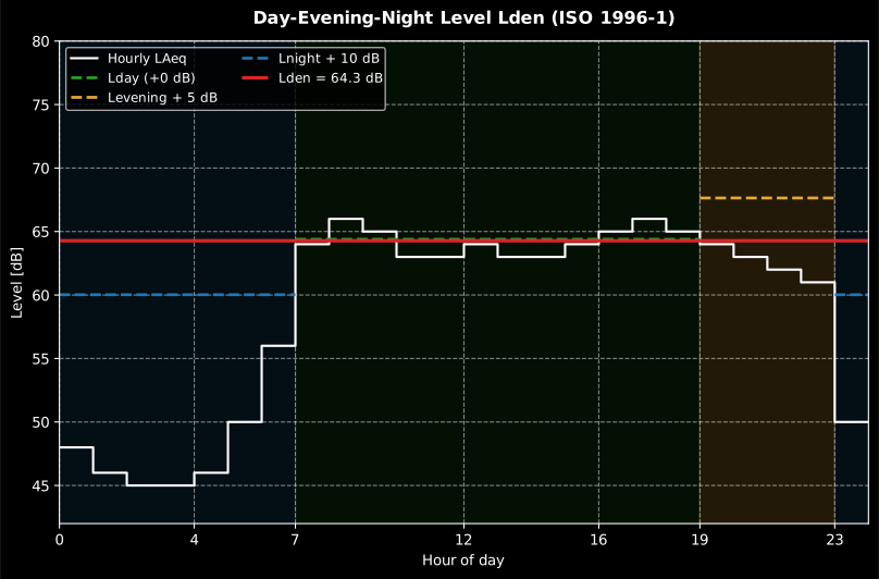
Regulatory noise assessment weights evenings and nights more heavily.
`lden()` implements the day-evening-night level of ISO 1996-1:2016 (3.6.4:
+5 dB evening, +10 dB night, default 12/4/8 h periods, adjustable because
countries define them differently), `ldn()` the day-night variant (3.6.5),
and `composite_rating_level()` the general whole-day composite of clause 6.5
(Formulae 5-6) for arbitrary periods with source or character adjustments
(Table A.1: e.g. +5 dB regular impulsive, +12 dB highly impulsive, +3 to
+6 dB prominent tones):
```python
from phonometry import environmental
l = environmental.lden(63.2, 58.1, 51.4) # from LAeq per period
r = environmental.composite_rating_level([(63.2, 12, 0.0), # day
(58.1, 4, 5.0), # evening (+5)
(51.4, 8, 10.0)]) # night (+10) == environmental.lden
```
Show the code for this figure
```python
import numpy as np
import matplotlib.pyplot as plt
from phonometry import environmental
# Synthetic hourly LAeq of an urban road (dB), hours 00 to 23
laeq_h = np.array([48, 46, 45, 45, 46, 50, 56, 64, 66, 65, 63, 63,
64, 63, 63, 64, 65, 66, 65, 64, 63, 62, 61, 50], dtype=float)
def period_leq(idx):
return 10 * np.log10(np.mean(10 ** (laeq_h[idx] / 10))) # energy mean
ld = period_leq(np.arange(7, 19)) # day 07-19
le = period_leq(np.arange(19, 23)) # evening 19-23
ln_ = period_leq(np.r_[23, np.arange(0, 7)]) # night 23-07
l_den = environmental.lden(ld, le, ln_)
print(f"Lden = {l_den:.1f} dB") # Lden = 64.3 dB
fig, ax = plt.subplots()
ax.axvspan(19, 23, color="C1", alpha=0.15) # evening
ax.axvspan(23, 24, color="C0", alpha=0.15); ax.axvspan(0, 7, color="C0", alpha=0.15)
ax.step(np.arange(25), np.r_[laeq_h, laeq_h[-1]], where="post",
color="0.3", label="Hourly LAeq")
ax.hlines(ld, 7, 19, color="C2", linestyle="--", label="Lday (+0 dB)")
ax.hlines(le + 5, 19, 23, color="C1", linestyle="--", label="Levening + 5 dB")
ax.hlines([ln_ + 10, ln_ + 10], [23, 0], [24, 7], color="C0",
linestyle="--", label="Lnight + 10 dB")
ax.hlines(l_den, 0, 24, color="C3", linewidth=2, label=f"Lden = {l_den:.1f} dB")
ax.set(xlabel="Hour of day", ylabel="Level [dB]", xlim=(0, 24))
ax.legend(loc="upper left", fontsize=8, ncol=2)
plt.show()
```
### `lden()` / `ldn()` / `composite_rating_level()` parameters
| Function | Key parameters | Notes |
| :--- | :--- | :--- |
| `lden(lday, levening, lnight, hours=(12, 4, 8))` | period LAeq values [dB]; `hours` must sum to 24 | +5 dB evening, +10 dB night (3.6.4) |
| `ldn(lday, lnight, hours=(15, 9))` | | +10 dB night (3.6.5) |
| `composite_rating_level(periods)` | iterable of `(level_db, hours, adjustment_db)`; hours positive, finite and summing to 24 | General Formulae (5)-(6); adjustments per Table A.1 |
Where you put the microphone changes the number: ISO 1996-2 fixes the receiver positions and their façade corrections. The diagram is measurement context; apply the corrections to your levels before analysis:
Combine with `laeq()` per time period to go from recordings to Lden, and with
the `tone_to_noise_ratio()` / `prominence_ratio()` verdicts of
[Prominent Discrete Tones](https://jmrplens.github.io/phonometry/guides/tone-prominence/) to justify tonal adjustments.
## Determining levels: tonal adjustment, residual noise and uncertainty (ISO 1996-2)
ISO 1996-2:2017 is the **determination** part: how the measured level is turned
into a rating level and reported with its uncertainty. The rating-level *summation*
and the time-of-day penalties live in ISO 1996-1 (above); ISO 1996-2 supplies the
tonal adjustment, the residual-noise correction and the uncertainty budget.
**Tonal adjustment (engineering method, Annex C).** From the energy-summed tone
level $L_{pt}$ and the masking-noise level $L_{pn}$ in the critical band around a
tone, the audibility above the masking threshold is
$\Delta L_{ta} = L_{pt} - L_{pn} + 2 + \lg[1 + (f_c/502)^{2.5}]$ dB (Formula (C.3)),
and the adjustment is $K_t = 0$ for $\Delta L_{ta} < 4$, $K_t = \Delta L_{ta} - 4$
for $4 \le \Delta L_{ta} \le 10$ and $K_t = 6$ above (Formulae (C.4)–(C.6)). The
critical bandwidth is 100 Hz up to 500 Hz and 20 % of $f_c$ above (Table C.1).
The one-third-octave **survey method** (`tonal_seeking_survey`) flags a band
exceeding both neighbours by 15/8/5 dB (low/mid/high), and
`tonal_adjustment_from_mean_audibility` maps the ISO/PAS 20065 mean audibility to
$K_t$ (Table J.1).
Show the code for this figure
```python
import matplotlib.pyplot as plt
from phonometry import environmental
# ISO 1996-2:2007 Annex C.5, Example 2 (two tones near 400 Hz):
res = environmental.assess_tonal_audibility(tone_level=54.1, masking_noise_level=45.2,
centre_frequency=430.0)
print(res.audibility, res.adjustment) # ΔLta ≈ 11.1 dB -> Kt = 6 dB
res.plot()
plt.show()
```
**Residual-noise correction (Clause 10.4).** `residual_sound_correction()`
applies $L = 10\lg(10^{L'/10} - 10^{L_\text{res}/10})$ (Formula (16)). With a
residual within 3 dB of the measured level no correction is allowed: the
*uncorrected* measured level $L'$ is then the reportable value, as an upper
bound of the specific sound (exposed as `reportable_upper_bound`, with
`reliable=False`). `gaussian_residual_level()` estimates the residual from
percentile levels (Annex I) and rejects inverted percentile orderings.
**Measurement uncertainty (Clause 4, Annex F).** `combined_standard_uncertainty()`
forms $u = \sqrt{\sum (c_j u_j)^2}$ (Formula (2)) and
`environmental_expanded_uncertainty()` applies $k = 2$ (95 %) or $k = 1.3$ (80 %);
`residual_correction_uncertainty()` carries the residual-correction sensitivity
(Formulae (F.7)/(F.8)) and `uncertainty_from_repeated_measurements()` the
repeated-measurement standard uncertainty: the primary energy-domain route
(Formulae (17)+(19)), with the level-domain Note 2 substitute (Formula (20))
reported alongside as `approximate_uncertainty` and a warning when the levels
spread beyond 3 dB, where the substitute grossly inflates.
```python
from phonometry import environmental
# Tonal adjustment for a prominent tone:
tonal = environmental.assess_tonal_audibility(54.1, 45.2, 430.0) # TonalAssessmentResult
kt = tonal.adjustment # 6 dB
tonal.plot() # this audibility on the Kt curve, as in the figure above
# Subtract residual (background) noise from a measured level:
corr = environmental.residual_sound_correction(measured_level=58.0, residual_level=50.0)
corr.corrected_level, corr.reliable
# Combine an uncertainty budget and expand to 95 %:
u = environmental.combined_standard_uncertainty([0.59, 0.3, 2.0, 0.40, 0.38]) # 2.18 dB (G.2)
environmental.expanded_uncertainty(u) # 4.36 dB (k = 2)
```
## Octave Spectrogram (levels over time)
Short-time fractional-octave analysis: one level per band per window,
time-aligned across bands.
```python
import numpy as np
from phonometry import metrology
# recording: a calibrated microphone capture (Pa) — recorded through your measurement chain. Synthesized here so the guide runs standalone.
fs = 48000
recording = 0.2 * np.sin(2 * np.pi * 1000 * np.arange(fs) / fs)
bank = metrology.OctaveFilterBank(fs=48000, fraction=3)
levels, freq, times = bank.spectrogram(recording, window_time=0.125, overlap=0.5)
# levels: (bands, frames) — ready for pcolormesh(times, freq, levels)
```
*A logarithmic sweep plus two tone bursts, resolved in time and in standardized
1/3-octave bands.*
Show the code for this figure
```python
import numpy as np
import matplotlib.pyplot as plt
from scipy.signal import chirp
from phonometry import metrology
# Log sweep 80 Hz -> 8 kHz plus two tone bursts, in a little noise
fs = 48000
t = np.arange(int(4.0 * fs)) / fs
x = 0.5 * chirp(t, f0=80, t1=4.0, f1=8000, method="logarithmic")
x[int(1.0 * fs):int(1.3 * fs)] += np.sin(2 * np.pi * 4000 * t[: int(0.3 * fs)])
x[int(2.5 * fs):int(2.8 * fs)] += np.sin(2 * np.pi * 250 * t[: int(0.3 * fs)])
x += 0.01 * np.random.default_rng(42).standard_normal(t.size)
bank = metrology.OctaveFilterBank(fs=fs, fraction=3, order=6, limits=[50.0, 12000.0])
levels, freq, times = bank.spectrogram(x, window_time=0.125, overlap=0.5)
fig, ax = plt.subplots()
mesh = ax.pcolormesh(times, freq, levels, shading="auto")
ax.set_yscale("log")
ax.set(xlabel="Time [s]", ylabel="Frequency [Hz]")
fig.colorbar(mesh, label="Level [dB]")
plt.show()
```
- Multichannel input `(channels, samples)` returns `(channels, bands, frames)`.
- `times` holds each window's center in seconds.
- `mode='peak'` gives per-window peak-holding levels instead of RMS.
- `zero_phase=True` filters bands forward-backward so per-band group delay does
not skew the frames (offline analysis only).
### `OctaveFilterBank.spectrogram()` parameters
| Parameter | Type | Units | Range / default | Notes |
| :--- | :--- | :--- | :--- | :--- |
| `x` | 1D or 2D array | digital units | non-empty | 2D returns `(channels, bands, frames)` |
| `window_time` | float | s | > 0; default `0.125` | Frame length (0.125 s mirrors Fast) |
| `overlap` | float | — | 0 ≤ overlap < 1; default `0.5` | Fraction of window overlap (0 = none) |
| `mode` | str | — | `'rms'` (default) or `'peak'` | Per-window detector |
| `detrend` | bool | — | default `True` | Remove each band's DC offset before the level (improves low-frequency accuracy) |
| `zero_phase` | bool | — | default `False` | Forward-backward filtering (offline only) |
| `calibration_factor` / `dbfs` | — | — | constructor-only | Set on `OctaveFilterBank(...)`, not per call |
See [Calibration and dBFS](https://jmrplens.github.io/phonometry/reference/api/levels/calibration/) to convert digital units to physical
SPL, and [Time Weighting](https://jmrplens.github.io/phonometry/guides/time-weighting/) for the envelope details. The
ISO 9612 occupational strategies continue in
[Occupational Noise Exposure](https://jmrplens.github.io/phonometry/reference/api/hearing/occupational-exposure/), the ECMA-418-1
tonal-prominence verdicts in [Prominent Discrete Tones](https://jmrplens.github.io/phonometry/guides/tone-prominence/),
and the ISO 226 equal-loudness contours live with the perception metrics in
[Loudness](https://jmrplens.github.io/phonometry/guides/loudness/).
## Quick answers
### What is the difference between Leq and SEL?
$L_{eq}$ is the equivalent continuous level: the energy mean of the squared
pressure over the measurement time $T$, referenced to
$p_0 = 20\ \mu\text{Pa}$. SEL, the sound exposure level ($L_{AE}$ when
A-weighted), compresses the whole event energy into exactly one second:
$L_E = L_{eq,T} + 10\log_{10}(T/T_0)$ with $T_0 = 1\ \text{s}$, so events of
any duration become directly comparable and $N$ identical events sum as
$+10\log_{10}N$.
### What sound exposure corresponds to 90 dB over an 8-hour working day?
Per IEC 61252:1993, the sound exposure $E$ is the time integral of the
squared A-weighted pressure, expressed in pascal-squared-hours, and
$L_{EX,8h}$ (equivalent to $L_{EP,d}$) is the corresponding level normalized
to 8 h. The anchor worth memorizing: 3.2 Pa²h corresponds to exactly 90 dB
over 8 h. Half the dose is -3 dB, and double duration at the same level is
+3 dB.
### What penalties does Lden apply to evening and night noise?
$L_{den}$, the day-evening-night level of ISO 1996-1:2016 (3.6.4), adds
+5 dB to the evening level and +10 dB to the night level before
energy-averaging the whole day, with default periods of 12, 4 and 8 hours,
adjustable because countries define them differently. The day-night variant
$L_{dn}$ (3.6.5) keeps only the +10 dB night penalty.
## References
- International Electrotechnical Commission. (2013). *Electroacoustics —
Sound level meters — Part 1: Specifications* (IEC 61672-1:2013).
[IEC webstore](https://webstore.iec.ch/en/publication/5708).
The envelope ballistics behind the percentile levels, the C-weighted peak
and the SEL toneburst references the implementation is verified against.
- Kinsler, L. E., Frey, A. R., Coppens, A. B., & Sanders, J. V. (2000).
*Fundamentals of acoustics* (4th ed.). Wiley. ISBN 978-0-471-84789-2.
[Publisher page](https://www.wiley.com/en-us/Fundamentals+of+Acoustics%2C+4th+Edition-p-9780471847892).
The sound-pressure, energy and level definitions underneath Leq, SEL and
the dose measures.
- British Standards Institution. (2003). *Description and measurement of
environmental noise — Guide to quantities and procedures* (BS 7445-1:2003).
[BSI Knowledge](https://knowledge.bsigroup.com/products/description-and-measurement-of-environmental-noise-guide-to-quantities-and-procedures).
The survey-practice companion of ISO 1996-1: which descriptor family fits
which assessment question (BS 7445-2:1991 covers the land-use data
acquisition).
- Bies, D. A., Hansen, C. H., & Howard, C. Q. (2017). *Engineering noise
control* (5th ed.). CRC Press.
[doi:10.1201/9781351228152](https://doi.org/10.1201/9781351228152).
Section 2.5 (the noise measures: Leq, Ldn, L10/L90 and their intended
uses) and Section 2.15 (environmental noise surveys). ISBN
978-1-4987-2405-0.
## Standards
IEC 61672-1:2013, *Electroacoustics — Sound level meters —
Part 1: Specifications*: the Fast/Slow/Impulse envelope ballistics behind
`ln_levels`, the C-weighted peak of §5.13 (verified against the Table 5 tone
bursts) and the sound exposure level verified against the Table 4 LAE column.
IEC 61252, *Electroacoustics — Specifications for personal sound exposure
meters*: the sound exposure E in Pa²h and the normalized 8 h level LEX,8h
(≡ LEP,d), anchored at 3.2 Pa²h ⇔ exactly 90 dB. ISO 1996-1:2016, *Acoustics —
Description, measurement and assessment of environmental noise — Part 1:
Basic quantities and assessment procedures*: Lden (3.6.4), Ldn (3.6.5) and
the composite whole-day rating level of clause 6.5 (Formulae 5-6, Table A.1
adjustments).