Source: https://jmrplens.github.io/phonometry/guides/insulation-field/
# Field Insulation Measurement and Ratings
This guide continues from the [Room Acoustics guide](https://jmrplens.github.io/phonometry/reference/api/rooms/room-acoustics/):
the same impulse response, measured either side of a partition, yields its sound
insulation. This page covers insulation measured *in the building*: field
airborne, impact and façade insulation with single-number ratings
(ISO 16283-1/2/3, ISO 717-1/2), the measurement uncertainty that qualifies
every rating (ISO 12999-1) and the quick ISO 10052 survey method. The
laboratory characterisation of an element lives in
[Laboratory Insulation Measurement](https://jmrplens.github.io/phonometry/guides/insulation-lab/) and the prediction of
in-situ performance in
[Predicting Sound Insulation (EN 12354)](https://jmrplens.github.io/phonometry/guides/insulation-prediction/).
## Field insulation and single-number ratings (ISO 16283-1, ISO 717-1)
To rate a wall or floor, measure the energy-average level in the **source**
room ($L_1$) and the **receiving** room ($L_2$) per one-third-octave band
and form the level difference $D = L_1 - L_2$. Two normalisations make it
comparable between rooms. The **standardized level difference** references
the receiving-room reverberation time $T$ to $T_0 = 0.5$ s (so with
$T = 0.5$ s, $D_{nT} = D$ exactly), and the **apparent sound reduction
index** normalises by the partition area $S$ and the Sabine absorption area
$A$:
$$
D_{nT} = D + 10 \log_{10} \frac{T}{T_0}, \qquad
R' = D + 10 \log_{10} \frac{S}{A}, \qquad A = \frac{0.16\ V}{T}.
$$
Positions are energy-averaged with
$L = 10 \log_{10}\left( \frac{1}{n} \sum_i 10^{L_i/10} \right)$.
The prime on $R'$ is a convention, not decoration: primed quantities ($R'$,
$L'_n$, $L'_{nT}$) are measured **in the building** and include every
flanking path, while the unprimed $R$ and $L_n$ are laboratory properties of
the element alone, measured with flanking suppressed. The full lab-to-field
map lives in [Laboratory Insulation Measurement](https://jmrplens.github.io/phonometry/guides/insulation-lab/); the
prediction that bridges the two is
[EN 12354](https://jmrplens.github.io/phonometry/guides/insulation-prediction/).
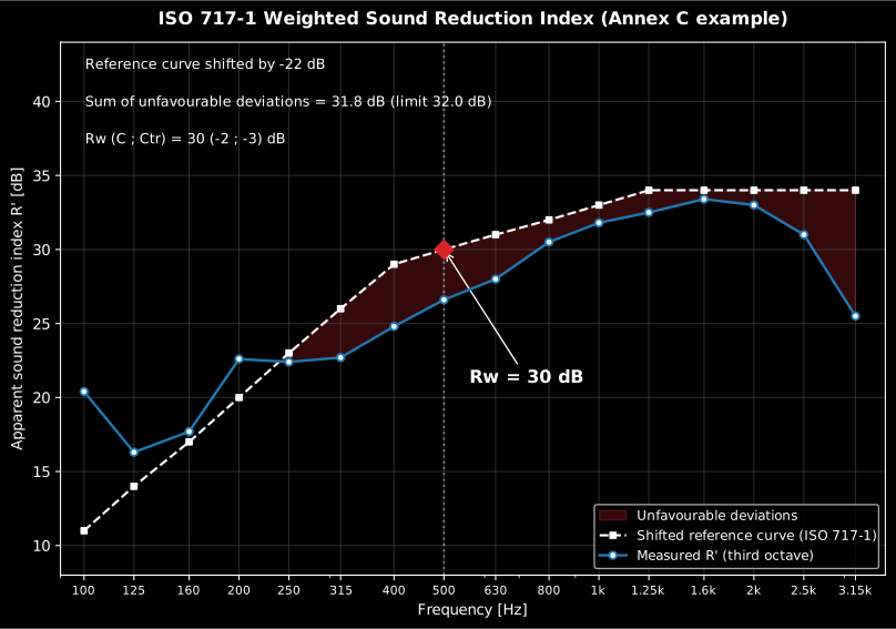
The band spectrum is collapsed to one number by the **reference-curve
method** of ISO 717-1: a fixed reference curve is shifted in 1 dB steps
toward the measured curve until the sum of *unfavourable* deviations
(where the measurement falls below the reference) is as large as possible
but not more than 32.0 dB (16 one-third-octave bands) or 10.0 dB (5 octave
bands). The rating (`Rw`, `R'w`, `DnT,w` …) is the shifted reference read at
500 Hz. The **spectrum adaptation terms** $C$ (pink noise) and $C_{tr}$
(urban traffic) add the low-frequency penalty of a real source.
The two terms re-rate the same measured curve against the two source spectra
of ISO 717-1 Annex A: $C$ against A-weighted pink noise, representative of
living activities (speech, music, radio, television), and $C_{tr}$ against
A-weighted urban road traffic, whose energy sits at low frequency. They are
defined so that the rating plus the term ($R_w + C$ for a laboratory index,
$R'_w + C$ or $D_{nT,w} + C$ for the field quantities of this guide, and
likewise with $C_{tr}$) is the A-weighted level difference achieved against
that source. Reading them:
* $C$ stays small for most constructions (0 to −2 dB is typical): the pink
spectrum is close to the weighting already implicit in the reference
curve.
* $C_{tr}$ punishes weak low-frequency insulation. A lightweight double leaf
with its mass-air-mass resonance near 100 Hz can carry a $C_{tr}$ of −5 to
−10 dB, while a heavy monolithic wall with the same $R_w$ loses far less:
two constructions with equal ratings can differ audibly against traffic.
* Design with the descriptor that matches the noise, carried by the field
quantity the requirement rates: $R'_w + C_{tr}$ for a façade on a busy
road, $D_{nT,w} + C$ (or the plain rating, where the regulation says so)
between dwellings, the two example requirements of ISO 717-1, 5.3.
```python
import numpy as np
from phonometry import building
# Energy-average several microphone positions in one room (dB)
print(round(float(building.energy_average_level([60.0, 66.0])), 1)) # 64.0
# Field insulation per band; area S and volume V add R'
l1 = np.full(16, 80.0) # source-room levels
l2 = np.full(16, 40.0) # receiving-room levels
t2 = np.full(16, 0.5) # receiving-room T (s)
ins = building.airborne_insulation(l1, l2, t2, area=10.0, volume=50.0)
print(round(float(ins.dnt[0]), 1)) # 40.0 (= D since T = T0)
print(round(float(ins.r_prime[0]), 1)) # 38.0
# Single-number rating from a measured 16-band R spectrum (ISO 717-1 Annex C)
R = [20.4, 16.3, 17.7, 22.6, 22.4, 22.7, 24.8, 26.6,
28.0, 30.5, 31.8, 32.5, 33.4, 33.0, 31.0, 25.5]
w = building.weighted_rating(R)
print(w.rating, w.c, w.ctr) # 30 -2 -3 -> Rw(C;Ctr) = 30(-2;-3)
w.plot() # measured R' vs shifted ISO 717-1 reference, deviations shaded (needs matplotlib)
```
Show the code for this figure
```python
import matplotlib.pyplot as plt
from phonometry import building
# Single-number rating from a measured 16-band R spectrum (ISO 717-1 Annex C)
R = [20.4, 16.3, 17.7, 22.6, 22.4, 22.7, 24.8, 26.6,
28.0, 30.5, 31.8, 32.5, 33.4, 33.0, 31.0, 25.5]
w = building.weighted_rating(R)
# One line — measured curve vs the shifted ISO 717-1 reference, deviations shaded:
w.plot()
plt.show()
# By hand, from the band curve the result now carries:
fig, ax = plt.subplots()
ax.semilogx(w.band_centers, w.measured, "o-", label="Measured R'")
ax.semilogx(w.band_centers, w.shifted_reference, "s--", label="Shifted reference")
ax.fill_between(w.band_centers, w.measured, w.shifted_reference,
where=w.measured < w.shifted_reference, interpolate=True,
alpha=0.3, label="Unfavourable deviations")
ax.set_xlabel("Frequency [Hz]")
ax.set_ylabel("Sound reduction index [dB]")
ax.set_title(f"Rw = {w.rating} dB (C={w.c:+d}; Ctr={w.ctr:+d})")
ax.legend()
plt.show()
```
Compute `l1`, `l2` and `t2` on the same 16 one-third-octave bands from
100 Hz to 3150 Hz (obtain `t2` from
`room_parameters(ir, fs, limits=(100, 3150), fraction=3).t30`, for example) and
pass them to `airborne_insulation`. Feed that function's `dnt` (or `r_prime`)
spectrum to `weighted_rating`, so every band aligns index-by-index with the
ISO 717-1 reference curve.
### `airborne_insulation()` parameters
| Parameter | Type | Units | Range / default | Notes |
| :--- | :--- | :--- | :--- | :--- |
| `l1` | 1D or 2D array | dB | one/band, or `(positions, bands)` | Source-room levels (2D is energy-averaged) |
| `l2` | 1D or 2D array | dB | same band count | Receiving-room levels |
| `t2` | 1D array | s | > 0, one per band | Receiving-room reverberation time |
| `area` | float, optional | m² | > 0, with `volume` | Partition area `S` (enables `R'`) |
| `volume` | float, optional | m³ | > 0, with `area` | Receiving-room volume `V` |
| `t0` | float | s | default `0.5` | Reference reverberation time `T0` |
### `weighted_rating()` parameters
| Parameter | Type | Units | Range / default | Notes |
| :--- | :--- | :--- | :--- | :--- |
| `values_by_band` | 1D array | dB | 16 (thirds) or 5 (octaves) | Measured `R`, `R'`, `DnT` … per band |
| `bands` | str or `None` | — | `'third-octave'` / `'octave'` / `None` | `None` infers from the count |
`airborne_insulation()` returns an `AirborneInsulationResult` (`d`, `dnt`,
`r_prime` or `None`); `weighted_rating()` returns a `WeightedRatingResult`
(`rating`, `c`, `ctr`, `unfavourable_sum`, all integers except the sum).
### Enlarged frequency ranges and one-decimal ratings
When the measurement covers more than the core 100–3150 Hz bands, ISO 717-1
Annex B defines additional adaptation terms with the range as a subscript
($C_{50\text{–}3150}$, $C_{50\text{–}5000}$, $C_{100\text{–}5000}$ and the
$C_{tr}$ counterparts), computed with the Table B.1 spectra over the enlarged
range. `weighted_rating_extended` takes the band values *with their centre
frequencies* and returns the core rating plus every extended term the input
covers (the impact counterpart `weighted_impact_rating_extended` adds
$C_{I,50\text{–}2500}$). With `one_decimal=True` the reference curve shifts in
0.1 dB steps and all reductions keep one decimal: the variant ISO 717
prescribes "for the expression of uncertainty" and ISO 12999-1 Annex B
requires when stating the uncertainty of a single-number value.
```python
from phonometry import building
# Single-number rating from a measured 16-band R spectrum (ISO 717-1 Annex C)
R = [20.4, 16.3, 17.7, 22.6, 22.4, 22.7, 24.8, 26.6,
28.0, 30.5, 31.8, 32.5, 33.4, 33.0, 31.0, 25.5]
freqs = [50, 63, 80, 100, 125, 160, 200, 250, 315, 400, 500,
630, 800, 1000, 1250, 1600, 2000, 2500, 3150, 4000, 5000]
r_ext = [18.7, 19.2, 20.0, *R, 26.8, 29.2] # ISO 717-1 Annex C, Table C.2
ext = building.weighted_rating_extended(r_ext, freqs)
print(ext.rating, ext.c, ext.ctr, ext.c_50_5000, ext.ctr_50_5000)
# 30 -2 -3 -2 -4 -> Rw(C;Ctr;C50-5000;Ctr,50-5000) = 30(-2;-3;-2;-4)
one_dp = building.weighted_rating_extended(r_ext, freqs, one_decimal=True)
print(one_dp.rating) # 30.0, the 0.1 dB-step rating for uncertainty statements
ext.plot() # enlarged-range curve vs the shifted core reference, Annex B terms in the title (needs matplotlib)
```
*The rating itself is still evaluated on the 16 core bands (100–3150 Hz);
the enlarged bands only enter the Annex B adaptation terms, so the shifted
reference curve stops at the core-range edges while the measured curve
continues into the shaded enlarged range.*
Show the code for this figure
```python
import matplotlib.pyplot as plt
from phonometry import building
# Single-number rating from a measured 16-band R spectrum (ISO 717-1 Annex C)
R = [20.4, 16.3, 17.7, 22.6, 22.4, 22.7, 24.8, 26.6,
28.0, 30.5, 31.8, 32.5, 33.4, 33.0, 31.0, 25.5]
freqs = [50, 63, 80, 100, 125, 160, 200, 250, 315, 400, 500,
630, 800, 1000, 1250, 1600, 2000, 2500, 3150, 4000, 5000]
r_ext = [18.7, 19.2, 20.0, *R, 26.8, 29.2] # ISO 717-1 Annex C, Table C.2
ext = building.weighted_rating_extended(r_ext, freqs)
# One line — the enlarged-range curve vs the shifted core reference:
ext.plot()
plt.show()
# By hand, from the band curves the result carries (the full enlarged-range
# curve on ext, the core-band reference on ext.core):
fig, ax = plt.subplots()
ax.semilogx(ext.band_centers, ext.measured, "o-", label="Measured R")
ax.semilogx(ext.core.band_centers, ext.core.shifted_reference, "s--",
label="Shifted reference (core bands)")
ax.fill_between(ext.core.band_centers, ext.core.measured,
ext.core.shifted_reference,
where=ext.core.measured < ext.core.shifted_reference,
interpolate=True, alpha=0.3, label="Unfavourable deviations")
ax.set_xlabel("Frequency [Hz]")
ax.set_ylabel("Sound reduction index [dB]")
ax.set_title(f"Rw = {ext.rating} dB (C50-5000={ext.c_50_5000:+g}; "
f"Ctr,50-5000={ext.ctr_50_5000:+g})")
ax.legend()
plt.show()
```
### Impact sound (ISO 16283-2, ISO 717-2)
Footstep noise is rated the other way round. Instead of how much a floor
*blocks*, impact insulation measures how much a standardized **tapping
machine** on the floor above puts into the room below, so a *higher* number
is *worse*. The energy-average impact sound pressure level $L_i$ in the
receiving room is normalised like the airborne case, but with a sign flip on
the reverberation term:
$$
L'_{nT} = L_i - 10 \log_{10} \frac{T}{T_0}, \qquad
L'_n = L_i + 10 \log_{10} \frac{A}{A_0}, \quad
A_0 = 10\ \text{m}^2,\ A = \frac{0.16\ V}{T}.
$$
The **standardized** impact level $L'_{nT}$ ($T_0 = 0.5$ s for dwellings)
needs only the receiving-room $T$, so with $T = 0.5$ s it equals $L_i$; the
**normalized** level $L'_n$ (referenced to a 10 m² absorption area) also needs
the receiving-room volume. Note the **minus** sign: more reverberation
*lowers* $L'_{nT}$, opposite to the airborne $D_{nT}$.
The single-number rating (ISO 717-2) shifts the same style of reference curve,
but an **unfavourable deviation now occurs where the measurement *exceeds* the
reference** (impact noise is worse when higher), the sign opposite to
ISO 717-1. The rating (`Ln,w`, `L'n,w`, `L'nT,w`) is the shifted reference read
at 500 Hz; for octave bands it is then reduced by 5 dB. The spectrum
adaptation term $C_I = L_{n,\text{sum}} - 15 - L_{n,w}$ uses the energetic sum
over 100–2500 Hz (the first 15 thirds, excluding 3150 Hz) or 125–2000 Hz
(octaves).
For measurements extended down to 50 Hz,
`weighted_impact_rating_extended` additionally returns the enlarged-range
term $C_{I,50\text{–}2500}$ (A.2.1 NOTE), and with `one_decimal=True` the
0.1 dB-step rating used in uncertainty statements (it reproduces the printed
$L_{n,r,0,w} = 77.6$ dB and $C_{I,r,0} = -10.3$ dB of A.2.2).
```python
import numpy as np
from phonometry import building
# 16 one-third-octave impact levels Li (100 Hz - 3150 Hz), dB, from the
# ISO 717-2 Annex C worked example, and the receiving-room T per band.
li = np.array([62.1, 63.2, 63.5, 66.2, 68.5, 70.0, 71.7, 73.1,
73.8, 73.5, 73.8, 73.3, 73.1, 73.0, 72.4, 71.2])
t2 = np.full(16, 0.5)
imp = building.impact_insulation(li, t2, volume=50.0)
print(round(float(imp.l_n_t[0]), 1)) # 62.1 (= Li since T = T0)
print(round(float(imp.l_n[0]), 1)) # 64.1 normalized to A0 = 10 m^2
# Weighted impact rating + spectrum adaptation term CI (ISO 717-2)
res_imp = building.weighted_impact_rating(imp.l_n_t)
print(res_imp.rating, res_imp.ci, res_imp.unfavourable_sum) # 79 -11 28.0 -> L'nT,w(CI)=79(-11)
# Octave-band data carry the extra -5 dB reduction (Clause 4.3.2)
octave = np.array([65.3, 64.5, 58.0, 55.8, 43.0])
print(building.weighted_impact_rating(octave).rating) # 54
res_imp.plot() # measured L'nT vs shifted ISO 717-2 reference, measured-above shaded (needs matplotlib)
```
Show the code for this figure
```python
import matplotlib.pyplot as plt
import numpy as np
from phonometry import building
# 16 one-third-octave impact levels Li (100 Hz - 3150 Hz), dB, from the
# ISO 717-2 Annex C worked example, and the receiving-room T per band.
li = np.array([62.1, 63.2, 63.5, 66.2, 68.5, 70.0, 71.7, 73.1,
73.8, 73.5, 73.8, 73.3, 73.1, 73.0, 72.4, 71.2])
t2 = np.full(16, 0.5)
imp = building.impact_insulation(li, t2, volume=50.0)
# Weighted impact rating + spectrum adaptation term CI (ISO 717-2)
res_imp = building.weighted_impact_rating(imp.l_n_t)
# One line — measured L'nT vs the shifted ISO 717-2 reference (measured-above shaded):
res_imp.plot()
plt.show()
# By hand, from the band curve the result now carries (note the opposite sign:
# an unfavourable deviation is where the MEASURED level exceeds the reference).
# Here the input was l_n_t, so the rated quantity is the field level L'nT,w:
fig, ax = plt.subplots()
ax.semilogx(res_imp.band_centers, res_imp.measured, "o-", label="Measured L'nT")
ax.semilogx(res_imp.band_centers, res_imp.shifted_reference, "s--", label="Shifted reference")
ax.fill_between(res_imp.band_centers, res_imp.shifted_reference, res_imp.measured,
where=res_imp.measured > res_imp.shifted_reference, interpolate=True,
alpha=0.3, label="Unfavourable deviations")
ax.set_xlabel("Frequency [Hz]")
ax.set_ylabel("Impact sound pressure level [dB]")
ax.set_title(f"L'nT,w = {res_imp.rating} dB (CI={res_imp.ci:+d})")
ax.legend()
plt.show()
```
Feed `impact_insulation`'s `l_n_t` (or `l_n`) straight into
`weighted_impact_rating`; the rating and `CI` reproduce the ISO 717-2 Annex C
values (thirds `L'nT,w = 79`, `CI = −11`; octave `54`, `CI = 0`).
#### `impact_insulation()` parameters
| Parameter | Type | Units | Range / default | Notes |
| :--- | :--- | :--- | :--- | :--- |
| `li` | 1D or 2D array | dB | one/band, or `(positions, bands)` | Energy-average impact SPL (2D is averaged over positions) |
| `t2` | 1D array | s | > 0, one per band | Receiving-room reverberation time |
| `volume` | float, optional | m³ | > 0 | Receiving-room `V` (enables `L'n`) |
| `t0` | float | s | default `0.5` | Reference reverberation time `T0` |
#### `weighted_impact_rating()` parameters
| Parameter | Type | Units | Range / default | Notes |
| :--- | :--- | :--- | :--- | :--- |
| `values_by_band` | 1D array | dB | 16 (thirds) or 5 (octaves) | Measured `Ln`, `L'n` or `L'nT` per band |
| `bands` | str or `None` | — | `'third-octave'` / `'octave'` / `None` | `None` infers from the count |
`impact_insulation()` returns an `ImpactInsulationResult` (`l_n_t`, `l_n` or
`None`); `weighted_impact_rating()` returns an `ImpactRatingResult` (`rating`,
`ci` integers, `unfavourable_sum` in dB).
### ISO 717 report (`.report()`)
Both rating results render a one-page PDF fiche laid out like an
accredited-laboratory test report through a `report(path)` method: a
standard-basis line (measurement standard plus the ISO 717 rating part), an
optional metadata header block, the one-third-octave table beside the
measured-versus-shifted-reference plot (the result's own `.plot()`), the boxed
single-number result, an optional verdict row and a footer with the fixed
disclaimer. `WeightedRatingResult.report()` labels the airborne ISO 717-1 fiche
(`Rw (C; Ctr)`, deviations where the reference is above the measurement);
`ImpactRatingResult.report()` labels the impact ISO 717-2 fiche (`Ln,w (CI)`,
deviations the opposite way). `SoundReductionResult.report()` is a convenience
that rates the predicted `R(f)` and writes its fiche in one call.
The report metadata is supplied as a `ReportMetadata` frozen dataclass (every
field optional; only the supplied fields are rendered, and the numeric fields
must be finite and positive). Passing `metadata=None` produces a lightweight
prediction fiche (body, result and disclaimer only). When
`metadata.requirement` is set, a verdict row is added: an airborne rating passes
when it is at or above the requirement, an impact rating when it is at or below
it (a lower impact level is better). Setting `verbose=True` swaps the two-column
`f | value` table for the ISO 717 Annex C columns (frequency, measured value,
shifted reference, unfavourable deviation).
Rendering needs reportlab, kept out of the runtime dependencies as the optional
`phonometry[report]` extra (`pip install phonometry[report]`); a missing
reportlab raises a clear `ImportError` with the install command, and the plot
still needs matplotlib (`phonometry[plot]`). Only `engine="reportlab"` is
supported; any other engine raises `ValueError`. The fiche renders in English by
default; pass `language="es"` for a Spanish fiche (translated fixed strings and
a comma decimal separator), e.g.
`building.weighted_rating(R).report("Rw_fiche_es.pdf", language="es")`.
```python
from phonometry import building, ReportMetadata
# Airborne rating from a measured 16-band R spectrum (ISO 717-1)
R = [20.4, 16.3, 17.7, 22.6, 22.4, 22.7, 24.8, 26.6,
28.0, 30.5, 31.8, 32.5, 33.4, 33.0, 31.0, 25.5]
metadata = ReportMetadata(
specimen="200 mm reinforced-concrete wall",
client="Acoustic Test Client Ltd.",
area=10.0, mass_per_area=460.0,
source_volume=53.0, receiving_volume=51.0,
temperature=21.5, relative_humidity=45.0, pressure=101.3,
test_room="Transmission suite T1",
measurement_standard="ISO 10140-2",
test_date="2026-07-18",
laboratory="Phonometry Reference Laboratory",
operator="J. M. Requena-Plens",
report_id="PHN-2026-0042",
requirement=42.0, # adds the PASS/FAIL verdict row
)
building.weighted_rating(R).report(
"Rw_fiche.pdf", metadata=metadata
) # Rw (C; Ctr)
# Impact rating from a measured 16-band L'nT spectrum (ISO 717-2)
l_nt = [45.0, 47.0, 48.0, 49.0, 51.0, 52.0, 53.0, 54.0,
55.0, 56.0, 57.0, 58.0, 55.0, 52.0, 49.0, 46.0]
building.weighted_impact_rating(l_nt).report("Lnw_fiche.pdf") # Ln,w (CI)
```
Rendered examples of both fiches, regenerated with `make reports`, are kept in
the repository. Click either preview to open the PDF:
[](https://raw.githubusercontent.com/jmrplens/phonometry/main/.github/reports/iso717_airborne_example.pdf)
*Airborne rating fiche (`WeightedRatingResult.report`), Rw (C; Ctr).*
[](https://raw.githubusercontent.com/jmrplens/phonometry/main/.github/reports/iso717_impact_example.pdf)
*Impact rating fiche (`ImpactRatingResult.report`), Ln,w (CI).*
#### Report metadata (`ReportMetadata`)
Every field is optional and only the supplied ones are rendered, so the same
object drives a full accredited fiche and a lightweight prediction fiche. The
numeric fields are validated on construction by physical range.
| Field | Type | Rendered as |
| --- | --- | --- |
| `specimen`, `client`, `mounted_by`, `manufacturer` | `str` | Header identity of the tested element and who it was tested for / mounted by |
| `area`, `mass_per_area` | `float > 0` | Sample area *S* (m²) and measured mass per unit area (kg/m²) |
| `source_volume`, `receiving_volume` | `float > 0` | Room volumes (m³) |
| `temperature`, `relative_humidity`, `pressure` | `float` | Single representative climate: air temperature (°C, any sign), relative humidity (0–100 %), ambient pressure (kPa, > 0) |
| `source_temperature`, `source_relative_humidity`, `receiving_temperature`, `receiving_relative_humidity` | `float` | Per-room climate when source and receiving rooms are reported separately (same ranges as above) |
| `test_room`, `mounting`, `measurement_standard`, `test_date` | `str` | Facility, mounting condition, the measurement standard (forms the standard-basis line) and the test date |
| `laboratory`, `operator`, `report_id`, `notes` | `str` | Footer: institute, operator signature line, report number and free-form remarks |
| `requirement` | `float > 0` | Target single number; adds the verdict row (airborne passes at or above it, impact at or below it) |
### ISO 16283 field test report (`.report()`)
The per-band field results write the test report of ISO 16283-1:2014 /
ISO 16283-2:2020 Clause 14 directly, laid out like the recommended results
forms (Annex B / Annex C) and the accredited field reports built on them.
`AirborneInsulationResult.report()` renders the standardized level difference
*DnT* fiche (Figure B.1) or, with `quantity="r_prime"`, the apparent sound
reduction index *R'* fiche (Figure B.2); `ImpactInsulationResult.report()`
renders the standardized *L'nT* fiche (Figure C.1) or, with `quantity="l_n"`,
the normalized *L'n* fiche (Figure C.2). Each fiche names the field standard
in its basis line, evaluates the ISO 717-1 / ISO 717-2 single-number rating
over the 16 core one-third-octave bands (100-3150 Hz), states the quantity to
one decimal place both in tabular form and as a curve against the shifted
reference curve (Clause 12), boxes the field rating (`DnT,w (C; Ctr)`,
`R'w (C; Ctr)`, `L'nT,w (CI)` or `L'n,w (CI)`) and prints the mandatory
statement that the evaluation is based on field measurement results obtained
by an engineering method.
`verbose=True` swaps the two-column table for the per-band measurement chain
(the energy-average *L1* and *L2*, or *Li*, and the reverberation time *T*
beside the reported quantity), the content accredited field reports annex; it
needs a result built by `airborne_insulation()` / `impact_insulation()`, which
retain those inputs on the result (`l1`, `l2`/`li`, `t2`, `t0`). Metadata, the
requirement verdict (airborne passes at or above it, impact at or below it),
`language="es"` and the `phonometry[report]` extra behave exactly as in the
ISO 717 fiche above.
```python
import numpy as np
from phonometry import building, ReportMetadata
# Field airborne: source/receiving levels and T per one-third-octave band
l1 = np.array([92.3, 93.1, 94.0, 94.4, 94.8, 95.0, 95.2, 95.4,
95.3, 95.1, 94.8, 94.4, 93.9, 93.3, 92.5, 91.6])
l2 = l1 - np.array([38.2, 40.1, 42.6, 45.2, 47.8, 50.1, 52.3, 54.0,
55.6, 57.1, 58.2, 59.0, 59.6, 60.1, 60.3, 59.8])
t2 = np.array([0.62, 0.58, 0.55, 0.53, 0.52, 0.50, 0.49, 0.48,
0.47, 0.46, 0.45, 0.45, 0.44, 0.43, 0.43, 0.42])
field = building.airborne_insulation(l1, l2, t2, area=12.5, volume=30.4)
field.plot() # per-band DnT (and R') of the measured chain (needs matplotlib)
metadata = ReportMetadata(
specimen="Separating wall, 240 mm brick with independent lining",
client="Example client",
area=12.5, source_volume=32.1, receiving_volume=30.4,
test_room="Dwelling A living room to dwelling B living room",
test_date="2026-07-20",
laboratory="Phonometry Reference Laboratory",
report_id="PHN-2026-0143",
requirement=50.0, # DnT,w >= 50 dB -> PASS/FAIL row
)
field.report("DnTw_field.pdf", metadata=metadata) # DnT,w (C; Ctr)
field.report("Rpw_field.pdf", quantity="r_prime",
metadata=metadata) # R'w (C; Ctr)
field.report("DnTw_chain.pdf", metadata=metadata,
verbose=True) # f | L1 | L2 | T | DnT
# Field impact: tapping-machine levels in the receiving room
li = np.array([58.0, 60.5, 62.0, 63.5, 65.0, 66.0, 66.5, 66.0,
65.5, 65.0, 64.0, 62.0, 59.0, 56.0, 53.0, 50.0])
imp = building.impact_insulation(li, t2, volume=30.4)
imp.report("LnTw_field.pdf",
metadata=ReportMetadata(requirement=58.0)) # L'nT,w (CI)
```
*The receiving-room reverberation time turns the raw level difference `D`
into the standardized `DnT` band by band; with `T` above `T0 = 0.5 s`
across the range, the correction lifts the curve slightly. The rating box
carries both single numbers of this measurement, `DnT,w` and `R'w`.*
Show the code for this figure
```python
import matplotlib.pyplot as plt
import numpy as np
from phonometry import building
# Field airborne: source/receiving levels and T per one-third-octave band
l1 = np.array([92.3, 93.1, 94.0, 94.4, 94.8, 95.0, 95.2, 95.4,
95.3, 95.1, 94.8, 94.4, 93.9, 93.3, 92.5, 91.6])
l2 = l1 - np.array([38.2, 40.1, 42.6, 45.2, 47.8, 50.1, 52.3, 54.0,
55.6, 57.1, 58.2, 59.0, 59.6, 60.1, 60.3, 59.8])
t2 = np.array([0.62, 0.58, 0.55, 0.53, 0.52, 0.50, 0.49, 0.48,
0.47, 0.46, 0.45, 0.45, 0.44, 0.43, 0.43, 0.42])
field = building.airborne_insulation(l1, l2, t2, area=12.5, volume=30.4)
# One line — the per-band DnT (and R') of the measured chain:
field.plot()
plt.show()
# By hand, from the result's fields:
bands = [100, 125, 160, 200, 250, 315, 400, 500,
630, 800, 1000, 1250, 1600, 2000, 2500, 3150]
x = np.arange(len(bands))
w = building.weighted_rating(field.dnt)
fig, ax = plt.subplots()
ax.fill_between(x, field.d, field.dnt, alpha=0.2, label="10 lg(T/T0)")
ax.plot(x, field.d, "--o", label="D (level difference)")
ax.plot(x, field.dnt, "-s", label="DnT (standardized)")
ax.set_xticks(x, [str(b) for b in bands], rotation=45)
ax.set(xlabel="Frequency [Hz]", ylabel="Level difference [dB]",
title=f"DnT,w = {w.rating} dB (C={w.c:+d}; Ctr={w.ctr:+d})")
ax.legend()
plt.show()
```
Rendered examples of both field fiches, regenerated with `make reports`, are
kept in the repository. Click either preview to open the PDF:
[](https://raw.githubusercontent.com/jmrplens/phonometry/main/.github/reports/iso16283_airborne_example.pdf)
*Field airborne fiche (`AirborneInsulationResult.report`), DnT,w (C; Ctr).*
[](https://raw.githubusercontent.com/jmrplens/phonometry/main/.github/reports/iso16283_impact_example.pdf)
*Field impact fiche (`ImpactInsulationResult.report`), L'nT,w (CI).*
### Field façade insulation (ISO 16283-3)
The same source/receiver logic reaches the building **façade**, but now the
source is *outdoors*: a loudspeaker at 45° or the road traffic itself. Rather
than a level difference across an internal partition, ISO 16283-3 references the
receiving-room level $L_2$ to the level **2 m in front of the façade**
$L_{1,2m}$, giving the level difference $D_{2m}$ and, exactly as in the airborne
case, its standardized and normalized forms:
$$
D_{2m} = L_{1,2m} - L_2, \quad
D_{2m,nT} = D_{2m} + 10 \log_{10}\frac{T}{T_0}, \quad
D_{2m,n} = D_{2m} - 10 \log_{10}\frac{A}{A_0},
$$
with $T_0 = 0.5$ s, $A_0 = 10$ m² and $A = 0.16\ V/T$ (dwellings). When the
microphone sits **on the test element** (surface level $L_{1,s}$) the *element*
method also yields an apparent sound reduction index, carrying a fixed
angle-of-incidence correction: $-1.5$ dB for the 45° loudspeaker method,
$-3$ dB for the all-angle road-traffic method:
$$
R'_{45°} = L_{1,s} - L_2 + 10 \log_{10}\frac{S}{A} - 1.5, \qquad
R'_{tr,s} = L_{1,s} - L_2 + 10 \log_{10}\frac{S}{A} - 3.
$$
The façade quantity is airborne, so its single-number rating uses the
**ISO 717-1** reference curve through `weighted_rating` unchanged (Annex F).
```python
import numpy as np
from phonometry import building
# Outdoor level 2 m in front of the façade, receiving-room level and T per
# one-third-octave band; surface_level is the microphone on the test element.
l1_2m = np.full(16, 75.0) # L1,2m outdoors
l2 = np.full(16, 33.0) # receiving-room L2
t2 = np.full(16, 0.5) # receiving-room T (s)
fac = building.facade_insulation(l1_2m, l2, t2, volume=50.0, area=11.5,
surface_level=np.full(16, 78.0), method="loudspeaker")
print(round(float(fac.d_2m[0]), 1)) # 42.0 D2m = L1,2m - L2
print(round(float(fac.d_2m_nt[0]), 1)) # 42.0 (= D2m since T = T0)
print(round(float(fac.d_2m_n[0]), 1)) # 40.0 normalized to A0 = 10 m^2
print(round(float(fac.r_prime[0]), 1)) # 42.1 R'45deg (loudspeaker, -1.5 dB)
# The road-traffic element method carries the -3 dB all-angle correction instead
tr = building.facade_insulation(l1_2m, l2, t2, volume=50.0, area=11.5,
surface_level=np.full(16, 78.0), method="road_traffic")
print(round(float(tr.r_prime[0]), 1)) # 40.6 R'tr,s (traffic, -3 dB)
# The façade quantity is airborne: rate D2m,nT with the ISO 717-1 engine
print(building.weighted_rating(fac.d_2m_nt).rating) # 42 Dls,2m,nT,w
fac.plot() # per-band D2m,nT with D2m, D2m,n and R' overlaid (needs matplotlib)
```
*The four façade quantities of one measurement: the raw `D2m`, its
standardized and normalized forms, and the element `R'45°` carrying the
−1.5 dB angle-of-incidence correction. The rating box reads the single
number `Dls,2m,nT,w` obtained by feeding `D2m,nT` to the ISO 717-1 engine.*
Show the code for this figure
```python
import matplotlib.pyplot as plt
import numpy as np
from phonometry import building
# A dwelling façade, 45° loudspeaker method: outdoor level 2 m in front,
# receiving-room level and T per one-third-octave band.
bands = np.array([100, 125, 160, 200, 250, 315, 400, 500,
630, 800, 1000, 1250, 1600, 2000, 2500, 3150], float)
l1_2m = np.array([76.0, 77.0, 78.0, 78.5, 79.0, 79.0, 79.0, 79.0,
78.5, 78.0, 77.5, 77.0, 76.5, 76.0, 75.0, 74.0])
d2m = np.array([24.0, 25.5, 27.0, 28.5, 30.0, 31.5, 33.0, 34.5,
36.0, 37.0, 38.0, 38.5, 39.0, 39.0, 38.5, 38.0])
t2 = np.array([0.65, 0.62, 0.58, 0.55, 0.52, 0.50, 0.49, 0.48,
0.47, 0.46, 0.45, 0.44, 0.43, 0.43, 0.42, 0.42])
fac = building.facade_insulation(l1_2m, l1_2m - d2m, t2, volume=32.0,
area=10.8, surface_level=l1_2m + 3.0,
method="loudspeaker", frequencies=bands)
# One line — D2m,nT with D2m, D2m,n and R' overlaid per band:
fac.plot()
plt.show()
# By hand, from the result's fields:
w = building.weighted_rating(fac.d_2m_nt)
fig, ax = plt.subplots()
ax.semilogx(bands, fac.d_2m_nt, "-s", label="D2m,nT (standardized)")
ax.semilogx(bands, fac.d_2m, "--o", label="D2m")
ax.semilogx(bands, fac.d_2m_n, ":", label="D2m,n (normalized)")
ax.semilogx(bands, fac.r_prime, "-.", label="R'45°")
ax.set_xlabel("Frequency [Hz]")
ax.set_ylabel("Level difference / reduction index [dB]")
ax.set_title(f"Dls,2m,nT,w = {w.rating} dB (C={w.c:+d}; Ctr={w.ctr:+d})")
ax.legend()
plt.show()
```
`surface_level`, `area` and `volume` are all optional: with only `l1_2m`, `l2`
and `t2` the function returns `d_2m` and `d_2m_nt`; add `volume` for `d_2m_n`;
add `surface_level` **and** `area` **and** `volume` for `r_prime`. Positions are
energy-averaged with the surface-level formula (Clause 9.5.1); band levels are
assumed already corrected for background noise.
#### `facade_insulation()` parameters
| Parameter | Type | Units | Range / default | Notes |
| :--- | :--- | :--- | :--- | :--- |
| `l1_2m` | 1D or 2D array | dB | one/band, or `(positions, bands)` | Level 2 m in front of the façade `L1,2m` |
| `l2` | 1D or 2D array | dB | same band count | Receiving-room levels |
| `t2` | 1D array | s | > 0, one per band | Receiving-room reverberation time |
| `area` | float, optional | m² | > 0, with `surface_level`, `volume` | Test-element area `S` (enables `R'`) |
| `volume` | float, optional | m³ | > 0 | Receiving-room `V` (enables `D2m,n`; required for `R'`) |
| `surface_level` | 1D/2D array, optional | dB | same band count | Surface level `L1,s` on the element (enables `R'`) |
| `method` | str | — | `'loudspeaker'` (−1.5 dB) / `'road_traffic'` (−3 dB) | Angle-of-incidence correction of `R'` |
| `t0` | float | s | default `0.5` | Reference reverberation time `T0` |
| `frequencies` | 1D array, optional | Hz | — | Band centres carried on the result for plotting |
`facade_insulation()` returns a `FacadeInsulationResult` (`d_2m`, `d_2m_nt`,
`d_2m_n` or `None`, `r_prime` or `None`, `frequencies`); feed any 16-band façade
quantity to `weighted_rating` for its ISO 717-1 single number.
#### ISO 16283-3 field façade report (`.report()`)
`FacadeInsulationResult.report(path)` writes the one-page ISO 16283-3 field
façade test report: the standard-basis line, an optional metadata header, the
one-third-octave table beside the measured-versus-shifted-reference curve, the
boxed field rating `D2m,nT,w (C; Ctr)`, the engineering-method statement, an
optional requirement verdict (a level difference passes at or above it) and a
footer. `quantity="d_2m_nt"` (default) reports the standardized level
difference; `"d_2m_n"` the normalized one; `"r_prime"` the apparent sound
reduction index `R'45`. `verbose=True`, `metadata`, `language="es"` and the
`phonometry[report]` extra behave exactly as in the fiches above.
```python
fac.report("D2mnTw_facade.pdf") # D2m,nT,w (C; Ctr)
fac.report("Rp45_facade.pdf", quantity="r_prime") # R'45,w (C; Ctr)
```
[](https://raw.githubusercontent.com/jmrplens/phonometry/main/.github/reports/iso16283_facade_example.pdf)
*Field façade fiche (`FacadeInsulationResult.report`), D2m,nT,w (C; Ctr).*
## Measurement uncertainty (ISO 12999-1)
A rating without an uncertainty is only half a result. ISO 12999-1 does not
re-measure anything; it tabulates the **standard uncertainty** $u$ of every
sound-insulation quantity, derived from inter-laboratory tests, and prescribes
how to expand and combine it. Which standard deviation is $u$ depends on the
**measurement situation** (Clause 5.2):
| Situation | Meaning | Standard uncertainty $u$ |
| :--- | :--- | :--- |
| **A** | laboratory characterisation (ISO 10140) | reproducibility $\sigma_R$ |
| **B** | same location, different teams | in-situ $\sigma_{situ}$ |
| **C** | same location, same operator repeated | repeatability $\sigma_r$ |
The expanded uncertainty is $U = k\ u$ (Formula 2) with the coverage factor $k$
of Table 8. A two-sided interval $Y = y \pm U$ (Formula 3, $k = 1.96$ at 95 %)
*reports* a value; the **one-sided** factor ($k = 1.65$ at 95 %) *declares
conformity* with a requirement (Formulae 4/5).
```python
from phonometry import building
# Situation B (same building, different teams) -> the in-situ standard deviation.
print(building.single_number_uncertainty("r_w", "B")) # 0.9 dB (Table 3)
u = building.band_uncertainty("airborne", "B") # per-band u (Table 2)
print(len(u.frequencies), u.uncertainties[10]) # 21 1.1 (the 500 Hz band)
u.plot() # the per-band u(f) spectrum of Table 2 (needs matplotlib)
# Report R'w = 52 dB with a two-sided 95 % interval (k = 1.96, Table 8):
uv = building.uncertain_value(52.0, "rprime_w", "B") # aliases resolve to r_w
print(uv.coverage_factor, round(uv.expanded_uncertainty, 1)) # 1.96 1.8
print(round(uv.lower, 1), round(uv.upper, 1)) # 50.2 53.8 -> 52 ± 1.8 dB
# Declaring conformity uses the ONE-sided factor (k = 1.65): does R'w provably
# clear a 50 dB requirement?
uc = building.uncertain_value(52.0, "rprime_w", "B", one_sided=True)
print(building.satisfies_lower_requirement(52.0, uc.expanded_uncertainty, 50.0)) # True
```
Impact quantities offer situations B/C only (Table 4, no 500 Hz band in the 2020
edition), and $\Delta L$ only situation A. Descriptors are case-insensitive with
aliases (`rprime_w`/`dnt_w`→`r_w`, `lprime_n_w`→`ln_w`); combine independent
components in quadrature with `combine_uncertainties`, and reduce by $m$
independent measurements with `reduce_by_independent_measurements` ($u/\sqrt{m}$).
Show the code for this figure
```python
import matplotlib.pyplot as plt
from phonometry import building
# The same R'w = 52 dB reported in each situation with its two-sided 95 % U.
situations = ["A", "B", "C"]
vals = [building.uncertain_value(52.0, "r_w", s) for s in situations]
fig, ax = plt.subplots(figsize=(7, 4))
ax.errorbar(situations, [v.value for v in vals],
yerr=[v.expanded_uncertainty for v in vals],
fmt="o", capsize=8, color="tab:blue")
for s, v in zip(situations, vals):
ax.annotate(f"±{v.expanded_uncertainty:.1f}", (s, v.upper),
textcoords="offset points", xytext=(8, 4))
ax.set_ylabel("R'w [dB]"); ax.set_xlabel("Measurement situation")
ax.set_title("R'w = 52 dB with 95 % expanded uncertainty (ISO 12999-1)")
fig.tight_layout()
plt.show()
```
### `band_uncertainty()` / `single_number_uncertainty()` / `uncertain_value()` parameters
| Parameter | Type | Units | Range / default | Notes |
| :--- | :--- | :--- | :--- | :--- |
| `measurand` | str | — | `'airborne'` / `'impact'` / `'impact_reduction'` | Selects Table 2 / 4 / 6 |
| `quantity` | str | — | `'r_w'`, `'ln_w'`, `'delta_lw'` (+ aliases, `+c`/`+ctr` variants) | Single-number descriptor |
| `situation` | str | — | `'A'` / `'B'` / `'C'` | Measurement situation (Clause 5.2) |
| `value` | float | dB | — | Best estimate `y` to attach `U` to |
| `coverage` | float | — | default `0.95` | Confidence level (Table 8) |
| `one_sided` | bool | — | default `False` | One-sided factor for conformity checks |
| `upper_limit` | bool | — | default `False` | Select the σR95 upper limit (airborne, situation A) |
`band_uncertainty()` returns a `BandUncertainty` (`frequencies`,
`uncertainties`, `.to_arrays()`); `single_number_uncertainty()` a float;
`uncertain_value()` an `UncertainValue` (`value`, `standard_uncertainty`,
`coverage_factor`, `expanded_uncertainty`, `.lower`, `.upper`). The read-only
`COVERAGE_FACTORS` mapping exposes Table 8 keyed by `(confidence, one_sided)`.
## Field survey method (ISO 10052)
The engineering methods above buy accuracy with effort: swept microphones,
per-band reverberation times, careful background correction. For a quick check
in a dwelling, ISO 10052 defines a **survey (control) method**: octave bands, a
hand-held meter, and a single quantity, the **reverberation index**
`k = 10 lg(T/T0)` (`T0 = 0.5 s`), to carry the receiving-room correction. Every
survey quantity is then just an addition of `k`: the standardized level
difference `DnT = D + k`, the normalized `Dn = D + k + 10 lg(A0 T0 / (0.16 V))`,
the apparent `R' = D + k + 10 lg(S T0 / (0.16 V))` (using `V/7.5` for `S` where
that is larger), and, for impacts and façades, `L'nT = Li - k` and
`D2m,nT = D2m + k`. The clause references follow ISO 10052:2021; the formulas
and the reverberation-index table are identical in the harmonized
EN ISO 10052:2004+A1:2010.
The reverberation index is either **measured** (feed the reverberation time to
`reverberation_index(T)`) or, in a control survey, **estimated** from the room
type and volume with `estimate_reverberation_index(V, room)` (Table 4:
furnished `"kitchen"` / `"bathroom"` / `"furnished"`, or the unfurnished
construction classes `"a"`–`"h"` and the mixed `"a+e"`…`"d+h"`). A fourth
quantity unique to this method is **service-equipment noise** `LXY`: the
energy average of three A- or C-weighted positions.
```python
import numpy as np
from phonometry import building
# Octave-band levels (125-2000 Hz) and the measured receiving-room T.
l1 = np.array([88.0, 90.0, 92.0, 92.0, 90.0])
l2 = np.array([55.0, 51.0, 47.0, 41.0, 35.0])
k = building.reverberation_index([0.70, 0.60, 0.50, 0.45, 0.40]) # k = 10 lg(T/0.5)
res = building.survey_airborne_insulation(l1, l2, k, volume=50.0, area=12.0)
print(np.round(res.d_nt, 1)) # [34.5 39.8 45. 50.5 54. ] DnT = D + k
print(res.rating.rating, res.rating.c) # 49 -1 -> DnT,w (C)
print(res.r_prime_rating.rating) # 48 -> R'w
# No reverberation time measured? Estimate k from Table 4 (heavy walls, hard
# floor, 35-60 m3 -> class "g").
k_est = building.estimate_reverberation_index(50.0, "g")
print(k_est) # [4.5 5. 5.5 5.5 5.5]
# Service-equipment noise: energy average of three A-weighted positions.
se = building.survey_service_equipment_level([35.0, 30.0, 32.0], 3.0, volume=50.0)
print(round(float(se.l_xy), 1), round(float(se.l_xy_nt), 1)) # 32.8 29.8
res.plot() # DnT vs shifted ISO 717-1 reference (needs matplotlib)
```
*The reverberation index `k = 10 lg(T/T0)` shifts the raw level difference `D`
into the standardized `DnT`: up where the room is live (`T > T0`), down where
it is dead. The automatic rating is formed only for exactly 5 octave (or 16
one-third-octave) values.*
Show the code for this figure
```python
import matplotlib.pyplot as plt
import numpy as np
from phonometry import building
# Octave-band levels (125-2000 Hz) and the measured receiving-room T.
bands = [125, 250, 500, 1000, 2000]
l1 = np.array([88.0, 90.0, 92.0, 92.0, 90.0])
l2 = np.array([55.0, 51.0, 47.0, 41.0, 35.0])
k = building.reverberation_index([0.70, 0.60, 0.50, 0.45, 0.40]) # k = 10 lg(T/0.5)
res = building.survey_airborne_insulation(l1, l2, k, volume=50.0)
x = np.arange(len(bands))
fig, ax = plt.subplots()
ax.fill_between(x, res.d, res.d_nt, alpha=0.2, label="k = 10 lg(T/T0)")
ax.plot(x, res.d, "--o", label="D (level difference)")
ax.plot(x, res.d_nt, "-s", label="DnT (standardized)")
ax.set_xticks(x, [str(b) for b in bands])
ax.set(xlabel="Frequency [Hz]", ylabel="Level difference [dB]",
title=f"ISO 10052 survey method: DnT,w = {res.rating.rating} dB")
ax.legend()
plt.show()
```
### `survey_airborne_insulation()` and friends: parameters
| Parameter | Type | Units | Range / default | Notes |
| :--- | :--- | :--- | :--- | :--- |
| `l1` / `l2` | 1D or 2D array | dB | one/band, or `(positions, bands)` | Source / receiving (or outdoor `l1_2m`) levels |
| `li` | 1D or 2D array | dB | one/band, or `(positions, bands)` | Impact levels (energy-averaged over positions) |
| `reverberation_index` | scalar or 1D array | dB | one per band | `k` from `reverberation_index` or `estimate_reverberation_index`; `survey_service_equipment_level()` also accepts a scalar `k` |
| `volume` | float | m³ | > 0 | Receiving-room `V` (for `Dn` / `L'n` / `R'` / normalized) |
| `area` | float | m² | > 0 | Common-partition `S` (airborne `R'`; `V/7.5` rule applied) |
| `measurements` | array | dB | exactly 3 | Service-equipment positions (`survey_service_equipment_level`) |
| `room` | str | — | `"kitchen"`/`"bathroom"`/`"furnished"`/`"a"`–`"h"`/`"a+e"`… | `estimate_reverberation_index` room class (Table 4) |
`survey_airborne_insulation()` returns a `SurveyAirborneResult` (`d`, `d_nt`,
`d_n`, `r_prime`, `rating`, `r_prime_rating`); `survey_impact_insulation()` a
`SurveyImpactResult` (`l_i`, `l_nt`, `l_n`, `rating`);
`survey_facade_insulation()` a `SurveyFacadeResult`;
`survey_service_equipment_level()` a `SurveyServiceEquipmentResult` (`l_xy`,
`l_xy_nt`, `l_xy_n`).
### ISO 10052 survey reports (`.report()`)
The airborne, impact and façade survey results each carry a `.report(path)` that
writes the one-page ISO 10052 survey (control) method field report: the
standard-basis line naming ISO 10052 (octave bands), an optional metadata
header, the octave-band table beside the measured-versus-shifted-reference
curve, the boxed field rating (`DnT,w`/`R'w`, `L'nT,w` or `D2m,nT,w`), the
survey-method statement, an optional requirement verdict (level differences pass
at or above it, the impact level at or below it) and a footer. The airborne
result reports `quantity="dnt"` (default) or `"r_prime"`; `verbose=True`,
`metadata` and `language="es"` behave as in the fiches above.
```python
import numpy as np
res.report("DnTw_survey.pdf",
metadata=ReportMetadata(requirement=40.0)) # DnT,w (C; Ctr)
# Impact and façade surveys reuse the same k; li is the tapping-machine level
# in the room below, l1_2m the level 2 m in front of the façade.
li = np.array([66.0, 64.0, 62.0, 60.0, 55.0])
impact = building.survey_impact_insulation(li, k, volume=50.0)
impact.plot() # L'nT vs the shifted ISO 717-2 reference (needs matplotlib)
impact.report("LnTw_survey.pdf") # L'nT,w (CI)
l1_2m = np.array([76.0, 78.0, 79.0, 79.0, 77.0])
facade = building.survey_facade_insulation(l1_2m, l2, k, volume=40.0)
facade.report("D2mnTw_survey.pdf") # D2m,nT,w (C; Ctr)
```
*The impact survey applies the reverberation index with the opposite sign,
`L'nT = Li − k`: a live receiving room (`T > T0`) **lowers** the standardized
impact level. As in the airborne case, the automatic rating appears for
exactly 5 octave (or 16 one-third-octave) values.*
Show the code for this figure
```python
import matplotlib.pyplot as plt
import numpy as np
from phonometry import building
# Octave-band tapping-machine levels below the floor, and the measured T.
bands = [125, 250, 500, 1000, 2000]
li = np.array([66.0, 64.0, 62.0, 60.0, 55.0])
k = building.reverberation_index([0.70, 0.60, 0.50, 0.45, 0.40])
impact = building.survey_impact_insulation(li, k, volume=50.0)
# One line — L'nT vs the shifted ISO 717-2 reference:
impact.plot()
plt.show()
# By hand, showing the sign flip of the correction:
x = np.arange(len(bands))
fig, ax = plt.subplots()
ax.fill_between(x, impact.l_i, impact.l_nt, alpha=0.2, label="-k = -10 lg(T/T0)")
ax.plot(x, impact.l_i, "--o", label="Li (impact level)")
ax.plot(x, impact.l_nt, "-s", label="L'nT (standardized)")
ax.set_xticks(x, [str(b) for b in bands])
ax.set(xlabel="Frequency [Hz]", ylabel="Impact sound pressure level [dB]",
title=f"ISO 10052 survey method: L'nT,w = {impact.rating.rating} dB")
ax.legend()
plt.show()
```
Rendered examples of the survey fiches, regenerated with `make reports`, are
kept in the repository. Click a preview to open the PDF:
[](https://raw.githubusercontent.com/jmrplens/phonometry/main/.github/reports/iso10052_airborne_example.pdf)
*Survey airborne fiche (`SurveyAirborneResult.report`), DnT,w (C; Ctr).*
[](https://raw.githubusercontent.com/jmrplens/phonometry/main/.github/reports/iso10052_impact_example.pdf)
*Survey impact fiche (`SurveyImpactResult.report`), L'nT,w (CI).*
[](https://raw.githubusercontent.com/jmrplens/phonometry/main/.github/reports/iso10052_facade_example.pdf)
*Survey façade fiche (`SurveyFacadeResult.report`), D2m,nT,w (C; Ctr).*
## Quick answers
### What does DnT,w mean?
$D_{nT,w}$ is the weighted standardized level difference. Per
one-third-octave band, $D_{nT} = D + 10 \log_{10}(T/T_0)$ references the
receiving-room reverberation time $T$ to $T_0 = 0.5$ s, with
$D = L_1 - L_2$ the source-to-receiving level difference (ISO 16283-1).
The ISO 717-1 reference-curve method then collapses the 16 bands from
100 Hz to 3150 Hz into the single number read at 500 Hz.
### What is the difference between R and R' in sound insulation?
The prime marks where the measurement was made: primed quantities ($R'$,
$L'_n$, $L'_{nT}$) are measured in the building and include every flanking
path, while the unprimed $R$ and $L_n$ are laboratory properties of the
element alone, measured with flanking suppressed. In the field
(ISO 16283-1), $R' = D + 10 \log_{10}(S/A)$ with partition area $S$ and
Sabine absorption area $A = 0.16\ V/T$.
### What is the difference between the C and Ctr spectrum adaptation terms?
Both re-rate the same measured curve against the two source spectra of
ISO 717-1 Annex A: $C$ against A-weighted pink noise (living activities:
speech, music, radio, television) and $C_{tr}$ against A-weighted urban
road traffic, whose energy sits at low frequency. $C$ is typically 0 to
−2 dB, while a lightweight double leaf with a mass-air-mass resonance near
100 Hz can carry a $C_{tr}$ of −5 to −10 dB.
## References
- Hopkins, C. (2007). *Sound insulation*. Butterworth-Heinemann.
ISBN 978-0-7506-6526-1.
[doi:10.4324/9780080550473](https://doi.org/10.4324/9780080550473).
The comprehensive treatment of airborne and impact sound insulation:
the measurement chains, the statistics of rooms behind the field
quantities and the interpretation of the single-number ratings.
- Vigran, T. E. (2008). *Building acoustics*. CRC Press.
ISBN 978-0-415-42853-8.
[doi:10.1201/9781482266016](https://doi.org/10.1201/9781482266016).
A compact textbook companion for the sound-transmission physics behind
these measurements.
- International Organization for Standardization. (2020). *Acoustics —
Rating of sound insulation in buildings and of building elements — Part 1:
Airborne sound insulation* (ISO 717-1:2020).
[iso.org catalogue](https://www.iso.org/standard/77435.html).
The reference-curve rating and the spectrum adaptation terms interpreted
above.
- International Organization for Standardization. (2014). *Acoustics — Field
measurement of sound insulation in buildings and of building elements —
Part 1: Airborne sound insulation* (ISO 16283-1:2014).
[iso.org catalogue](https://www.iso.org/standard/55997.html).
The field airborne method this page implements.
## Standards
ISO 16283-1:2014, ISO 16283-2 and ISO 16283-3:2016, *Acoustics —
Field measurement of sound insulation in buildings and of building elements*:
the level differences, normalisations and element methods; ISO 717-1 and
ISO 717-2, which give the reference-curve single-number ratings and the spectrum
adaptation terms C, Ctr and CI; ISO 12999-1:2020, which tabulates the standard
uncertainties per measurement situation and the coverage factors; its precision framework
builds on ISO 5725 (context, not implemented directly); ISO 10052:2021
(harmonized as EN ISO 10052:2004+A1:2010), which defines the field survey method: the
reverberation-index correction, the standardized/normalized airborne, impact
and façade quantities, and service-equipment noise.
## See also
- [Laboratory Insulation Measurement](https://jmrplens.github.io/phonometry/guides/insulation-lab/): the
ISO 10140 element characterisation these field quantities are compared against.
- [Predicting Sound Insulation (EN 12354)](https://jmrplens.github.io/phonometry/guides/insulation-prediction/):
the in-situ performance predicted from laboratory element data.
- [Room Acoustics](https://jmrplens.github.io/phonometry/reference/api/rooms/room-acoustics/): the impulse response,
room parameters and sound absorption that this guide's insulation chain builds on.
- [Levels](https://jmrplens.github.io/phonometry/reference/api/levels/levels/): energy averaging and the level metrics behind
source/receiving-room levels.
- [Filter Banks](https://jmrplens.github.io/phonometry/guides/filter-banks/): the IEC 61260 fractional-octave filters
used for the insulation spectra.
- [Theory](https://jmrplens.github.io/phonometry/reference/theory/rooms-buildings/): the reference-curve derivation behind the
weighted single-number ratings.
- API reference: [`building.insulation`](https://jmrplens.github.io/phonometry/reference/api/building/insulation/), [`building.survey_insulation`](https://jmrplens.github.io/phonometry/reference/api/building/survey-insulation/) and [`building.building_uncertainty`](https://jmrplens.github.io/phonometry/reference/api/building/building-uncertainty/).